Computing backbone curves

Let us consider an autonomous dynamical mechanical system

$\mathbf{M\ddot{x}+C\dot{x}+Kx +f(x,\dot{x}) = 0}$

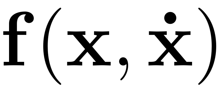
with nonlinear internal forces $\mathbf{f(x,\dot{x}})$ .

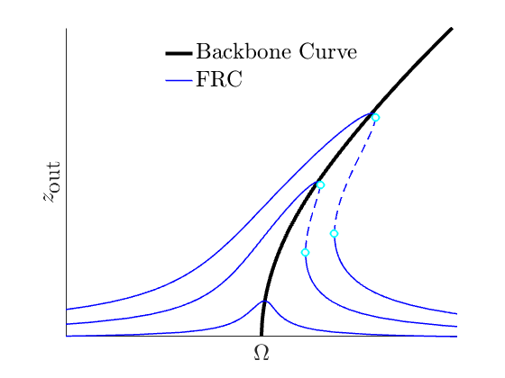
The backbone curve of such a system is defined as the collection of points which sit at the locus, ie. the point of maximal amplitude, of the nonlinear forced oscillations of a system. In this tutorial will motivate how such a curve can be obtained directly from the ROM provided by the reduced dynamics on a 2-dimensional SSM. In the following figure an illustration of a backbone curve is given, along with the forced response with various forcing amplitudes. Depending on the magnitude and characteristics of the nonlinear internal forces, the curve will bend in different ways, thus giving conclusive results about they system's nonlinear properties.

SSM Computation
Example
Linear Modal analysis and SSM setup
Setup SSM computation

SSM Computation

Assume we are interested in the nonlinear behaviour of the $i$ -th mode. Its linear response frequency is determined via the eigenvalue problem

$(\mathbf{M} \lambda_i^2+\mathbf{C} \lambda_i+\mathbf{K})\mathbf{v}_i= \mathbf{0}$

where the resonance frequency is $\omega_i = \textrm{Im}(\lambda_i)$ . Assume also that there are no outer resonances and procede with constructing a ROM on the autonomous SSM which is computed as a nonlinear continuation of $E_i = \textrm{span}(\mathbf{v}_i, \mathbf{\bar{v}}_i)$ . The following figure (cf. Jain & Haller, 2021) depicts how the manifold is embedded in the full space via the autonomous parametrisation $\mathbf{W(p)}$ of the invariant SSM.

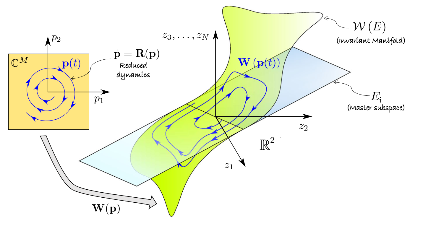
The reduced dynamics for such a system are given as

$\dot{\mathbf{p}} = \sum_{\mathbf{m}\in \mathbf{N}^2} \mathbf{R}_{\mathbf{m}} \mathbf{p}^{\mathbf m}$ .

To obtain an analytical expression for a backbone curve the parametrisation coordinates are transformed to polar notation. We set $$\mathbf{p} = [p, \bar{p}] = [\rho e^{i\theta}, \rho e^{-i\theta}]$ $ . In the new coordinates the reduced dynamics read

$\dot{\rho} = \textrm{Re} \bigg( \sum_{\mathbf{m}} R^1_{\mathbf{m}} \rho^{|\mathbf{m}|} \bigg)$

$\omega(\rho) = \dot{\theta} = \textrm{Im} \bigg( \sum_{\mathbf{m}} R^1_{\mathbf{m}} \rho^{|\mathbf{m}|-1} \bigg)$

For each polar amplitude a unique change in polar angle 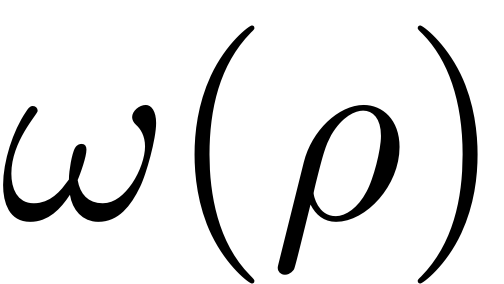$\omega(\rho)$ thus results. This prompts us to define the backbone curve in this context as the collection of points which follow this analytical relation (cf. Szalai, Erhardt & Haller 20017, Haller, Pedergnana & Ponsioen 2018).

Now consider a particular amplitude 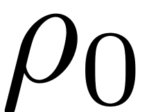$\rho_0$ in the polar parametrisation space. The amplitude of a corresponding nonlinear periodic orbit of the full nonlinear physical system which oscillates with frequency 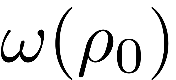$\omega(\rho_0)$ is then given by

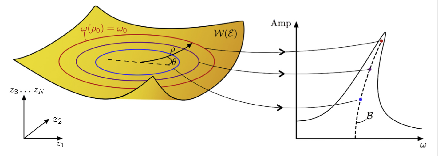
$\textrm{A}(\rho_0) = \frac{1}{2\pi} \int^{2\pi}_0 || \mathbf{W(p}(\rho_0,\theta))||_2 d\theta$ .

Thus, in the full system, the backbone curve computed on the SSM is given by the set $\{ \omega(\rho) , \textrm{A}(\rho) \}$ . A depiction of this process is shown in the following figure (cf. Ponsioen, Pedergnana & Haller 2018)

Example

As an example, we take the system of an <oscillatory chain.html > with cubic nonlinearities, as treated in our toolbox.

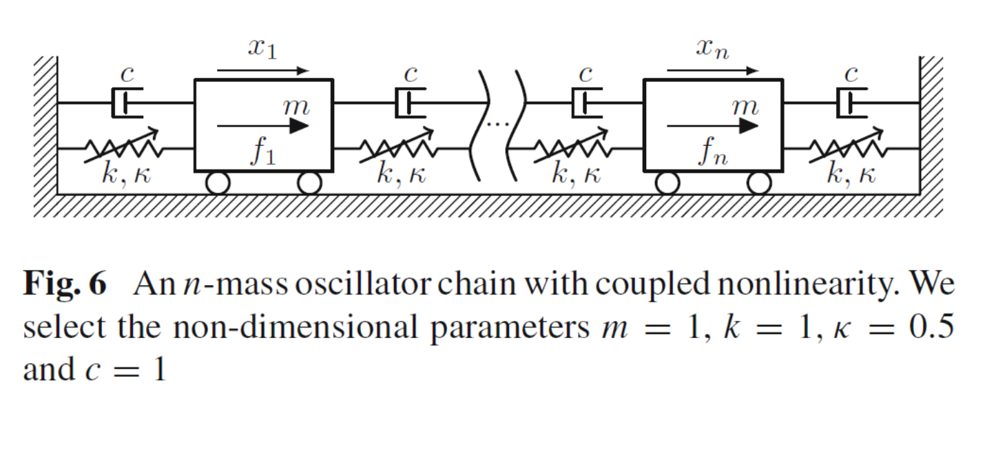
Setup

clear DS S
n = 10;
m = 1;
k = 1;
c = 0.1;
kappa2 = 0;
kappa3 = 0.5;

[M,C,K,fnl,~] = build_model(n,m,c,k,kappa2,kappa3);
DS = DynamicalSystem();
set(DS,'M',M,'C',C,'K',K,'fnl',fnl);
set(DS.Options,'Emax',5,'Nmax',10,'notation','multiindex')

To analyse the nonlinear forced response of the assume periodic forcing of the form

$\mathbf{f}^{ext}(\phi) = \mathbf{f}_0\cos(\phi)=\frac{\mathbf{f}_0}{2}e^{i\phi} + \frac{\mathbf{f}_0}{2}e^{-i\phi}$

with amplitued $\epsilon$ .

epsilon = 5e-3;
f_0 = ones(n,1);
kappas = [-1; 1];
coeffs = [f_0 f_0]/2;
DS.add_forcing(coeffs, kappas,epsilon);

Linear Modal analysis and SSM setup

[V,D,W] = DS.linear_spectral_analysis();

Due to high-dimensionality, we compute only the first 5 eigenvalues with the smallest magnitude. These would also be used to compute the spectral quotients
Assuming a proportional damping hypthesis with symmetric matrices
modal damping ratio for 1 mode is 1.423148e-02
modal damping ratio for 2 mode is 2.817326e-02
modal damping ratio for 3 mode is 4.154150e-02
modal damping ratio for 4 mode is 5.406408e-02
modal damping ratio for 5 mode is 6.548607e-02

 The first 10 nonzero eigenvalues are given as 
  -0.0041 + 0.2846i
  -0.0041 - 0.2846i
  -0.0159 + 0.5632i
  -0.0159 - 0.5632i
  -0.0345 + 0.8301i
  -0.0345 - 0.8301i
  -0.0585 + 1.0797i
  -0.0585 - 1.0797i
  -0.0858 + 1.3069i
  -0.0858 - 1.3069i

Choose Master subspace (perform resonance analysis)

S = SSM(DS);
set(S.Options, 'reltol', 0.1,'notation','multiindex')
masterModes = [1,2];
S.choose_E(masterModes);

(near) outer resonance detected for the following combination of master eigenvalues
     2     0
     3     1
     4     2
     5     3
     6     4
     0     2
     1     3
     2     4
     3     5
     4     6
     4     1
     5     2
     6     3
     1     4
     2     5
     3     6

These are in resonance with the follwing eigenvalues of the slave subspace
  -0.0159 + 0.5632i
  -0.0159 + 0.5632i
  -0.0159 + 0.5632i
  -0.0159 + 0.5632i
  -0.0159 + 0.5632i
  -0.0159 - 0.5632i
  -0.0159 - 0.5632i
  -0.0159 - 0.5632i
  -0.0159 - 0.5632i
  -0.0159 - 0.5632i
  -0.0345 + 0.8301i
  -0.0345 + 0.8301i
  -0.0345 + 0.8301i
  -0.0345 - 0.8301i
  -0.0345 - 0.8301i
  -0.0345 - 0.8301i

sigma_out = 21
(near) inner resonance detected for the following combination of master eigenvalues
     2     1
     3     2
     4     3
     1     2
     2     3
     3     4

These are in resonance with the follwing eigenvalues of the master subspace
  -0.0041 + 0.2846i
  -0.0041 + 0.2846i
  -0.0041 + 0.2846i
  -0.0041 - 0.2846i
  -0.0041 - 0.2846i
  -0.0041 - 0.2846i

sigma_in = 21

Setup SSM computation

We choose to use a continuation based approach to obtain the FRC directly from the ROM on the SSM. The following parameters are chosen for continuation.

order = 7; % Approximation order
outdof = floor(n/2);
set(S.Options, 'reltol', 1,'IRtol',0.02,'notation', 'multiindex')
set(S.FRCOptions, 'nt', 2^7,  'nPar', 100, 'outdof',outdof)
set(S.FRCOptions, 'method','continuation ep')
set(S.contOptions,'h0',0.01,'h_max',0.1)

choose frequency range

omega0 = imag(S.E.spectrum(1));
omegaRange = omega0*[0.8 1.2];
% Extract Backbone Curve

BB = S.extract_backbone(masterModes,omegaRange, order);

(near) outer resonance detected for the following combination of master eigenvalues
     2     0
     2     1
     3     1
     3     2
     4     2
     4     3
     5     3
     5     4
     6     4
     0     2
     1     2
     1     3
     2     3
     2     4
     3     4
     3     5
     4     5
     4     6
     2     0
     3     0
     3     1
     4     1
     4     2
     5     2
     5     3
     6     3
     6     4
     0     2
     0     3
     1     3
     1     4
     2     4
     2     5
     3     5
     3     6
     4     6
     3     0
     4     0
     4     1
     5     1
     5     2
     6     2
     6     3
     7     3
     0     3
     0     4
     1     4
     1     5
     2     5
     2     6
     3     6
     3     7
     4     0
     5     0
     5     1
     6     1
     6     2
     7     2
     7     3
     0     4
     0     5
     1     5
     1     6
     2     6
     2     7
     3     7

These are in resonance with the follwing eigenvalues of the slave subspace
  -0.0159 + 0.5632i
  -0.0159 + 0.5632i
  -0.0159 + 0.5632i
  -0.0159 + 0.5632i
  -0.0159 + 0.5632i
  -0.0159 + 0.5632i
  -0.0159 + 0.5632i
  -0.0159 + 0.5632i
  -0.0159 + 0.5632i
  -0.0159 - 0.5632i
  -0.0159 - 0.5632i
  -0.0159 - 0.5632i
  -0.0159 - 0.5632i
  -0.0159 - 0.5632i
  -0.0159 - 0.5632i
  -0.0159 - 0.5632i
  -0.0159 - 0.5632i
  -0.0159 - 0.5632i
  -0.0345 + 0.8301i
  -0.0345 + 0.8301i
  -0.0345 + 0.8301i
  -0.0345 + 0.8301i
  -0.0345 + 0.8301i
  -0.0345 + 0.8301i
  -0.0345 + 0.8301i
  -0.0345 + 0.8301i
  -0.0345 + 0.8301i
  -0.0345 - 0.8301i
  -0.0345 - 0.8301i
  -0.0345 - 0.8301i
  -0.0345 - 0.8301i
  -0.0345 - 0.8301i
  -0.0345 - 0.8301i
  -0.0345 - 0.8301i
  -0.0345 - 0.8301i
  -0.0345 - 0.8301i
  -0.0585 + 1.0797i
  -0.0585 + 1.0797i
  -0.0585 + 1.0797i
  -0.0585 + 1.0797i
  -0.0585 + 1.0797i
  -0.0585 + 1.0797i
  -0.0585 + 1.0797i
  -0.0585 + 1.0797i
  -0.0585 - 1.0797i
  -0.0585 - 1.0797i
  -0.0585 - 1.0797i
  -0.0585 - 1.0797i
  -0.0585 - 1.0797i
  -0.0585 - 1.0797i
  -0.0585 - 1.0797i
  -0.0585 - 1.0797i
  -0.0858 + 1.3069i
  -0.0858 + 1.3069i
  -0.0858 + 1.3069i
  -0.0858 + 1.3069i
  -0.0858 + 1.3069i
  -0.0858 + 1.3069i
  -0.0858 + 1.3069i
  -0.0858 - 1.3069i
  -0.0858 - 1.3069i
  -0.0858 - 1.3069i
  -0.0858 - 1.3069i
  -0.0858 - 1.3069i
  -0.0858 - 1.3069i
  -0.0858 - 1.3069i

sigma_out = 21
(near) inner resonance detected for the following combination of master eigenvalues
     2     1
     3     2
     4     3
     5     4
     1     2
     2     3
     3     4
     4     5

These are in resonance with the follwing eigenvalues of the master subspace
  -0.0041 + 0.2846i
  -0.0041 + 0.2846i
  -0.0041 + 0.2846i
  -0.0041 + 0.2846i
  -0.0041 - 0.2846i
  -0.0041 - 0.2846i
  -0.0041 - 0.2846i
  -0.0041 - 0.2846i

sigma_in = 21
Due to (near) outer resonance, the exisitence of the manifold is questionable and the underlying computation may suffer.
Attempting manifold computation
Manifold computation time at order 2 = 00:00:00
Estimated memory usage at order  2 = 1.70E-02 MB
Manifold computation time at order 3 = 00:00:00
Estimated memory usage at order  3 = 2.24E-02 MB
Manifold computation time at order 4 = 00:00:00
Estimated memory usage at order  4 = 3.25E-02 MB
Manifold computation time at order 5 = 00:00:00
Estimated memory usage at order  5 = 4.51E-02 MB
Manifold computation time at order 6 = 00:00:00
Estimated memory usage at order  6 = 6.22E-02 MB
Manifold computation time at order 7 = 00:00:00
Estimated memory usage at order  7 = 8.40E-02 MB
gamma = 
   0.0000 + 0.0024i
  -0.0000 - 0.0000i
  -0.0000 + 0.0000i

Total time spent on backbone curve computation = 00:00:01

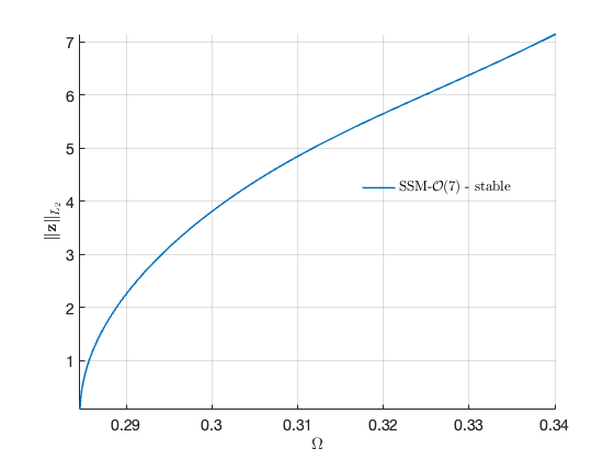
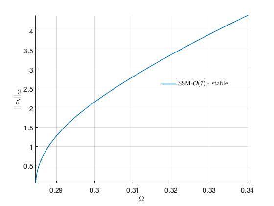
Extract Forced Response Curve

FRC = S.extract_FRC('freq',omegaRange,order);

*****************************************
Calculating FRC using SSM with master subspace: [1  2]
(near) outer resonance detected for the following combination of master eigenvalues
     2     0
     2     1
     3     1
     3     2
     4     2
     4     3
     5     3
     5     4
     6     4
     0     2
     1     2
     1     3
     2     3
     2     4
     3     4
     3     5
     4     5
     4     6
     2     0
     3     0
     3     1
     4     1
     4     2
     5     2
     5     3
     6     3
     6     4
     0     2
     0     3
     1     3
     1     4
     2     4
     2     5
     3     5
     3     6
     4     6
     3     0
     4     0
     4     1
     5     1
     5     2
     6     2
     6     3
     7     3
     0     3
     0     4
     1     4
     1     5
     2     5
     2     6
     3     6
     3     7
     4     0
     5     0
     5     1
     6     1
     6     2
     7     2
     7     3
     0     4
     0     5
     1     5
     1     6
     2     6
     2     7
     3     7

These are in resonance with the follwing eigenvalues of the slave subspace
  -0.0159 + 0.5632i
  -0.0159 + 0.5632i
  -0.0159 + 0.5632i
  -0.0159 + 0.5632i
  -0.0159 + 0.5632i
  -0.0159 + 0.5632i
  -0.0159 + 0.5632i
  -0.0159 + 0.5632i
  -0.0159 + 0.5632i
  -0.0159 - 0.5632i
  -0.0159 - 0.5632i
  -0.0159 - 0.5632i
  -0.0159 - 0.5632i
  -0.0159 - 0.5632i
  -0.0159 - 0.5632i
  -0.0159 - 0.5632i
  -0.0159 - 0.5632i
  -0.0159 - 0.5632i
  -0.0345 + 0.8301i
  -0.0345 + 0.8301i
  -0.0345 + 0.8301i
  -0.0345 + 0.8301i
  -0.0345 + 0.8301i
  -0.0345 + 0.8301i
  -0.0345 + 0.8301i
  -0.0345 + 0.8301i
  -0.0345 + 0.8301i
  -0.0345 - 0.8301i
  -0.0345 - 0.8301i
  -0.0345 - 0.8301i
  -0.0345 - 0.8301i
  -0.0345 - 0.8301i
  -0.0345 - 0.8301i
  -0.0345 - 0.8301i
  -0.0345 - 0.8301i
  -0.0345 - 0.8301i
  -0.0585 + 1.0797i
  -0.0585 + 1.0797i
  -0.0585 + 1.0797i
  -0.0585 + 1.0797i
  -0.0585 + 1.0797i
  -0.0585 + 1.0797i
  -0.0585 + 1.0797i
  -0.0585 + 1.0797i
  -0.0585 - 1.0797i
  -0.0585 - 1.0797i
  -0.0585 - 1.0797i
  -0.0585 - 1.0797i
  -0.0585 - 1.0797i
  -0.0585 - 1.0797i
  -0.0585 - 1.0797i
  -0.0585 - 1.0797i
  -0.0858 + 1.3069i
  -0.0858 + 1.3069i
  -0.0858 + 1.3069i
  -0.0858 + 1.3069i
  -0.0858 + 1.3069i
  -0.0858 + 1.3069i
  -0.0858 + 1.3069i
  -0.0858 - 1.3069i
  -0.0858 - 1.3069i
  -0.0858 - 1.3069i
  -0.0858 - 1.3069i
  -0.0858 - 1.3069i
  -0.0858 - 1.3069i
  -0.0858 - 1.3069i

sigma_out = 21
(near) inner resonance detected for the following combination of master eigenvalues
     2     1
     3     2
     4     3
     5     4
     1     2
     2     3
     3     4
     4     5

These are in resonance with the follwing eigenvalues of the master subspace
  -0.0041 + 0.2846i
  -0.0041 + 0.2846i
  -0.0041 + 0.2846i
  -0.0041 + 0.2846i
  -0.0041 - 0.2846i
  -0.0041 - 0.2846i
  -0.0041 - 0.2846i
  -0.0041 - 0.2846i

sigma_in = 21
Due to (near) outer resonance, the exisitence of the manifold is questionable and the underlying computation may suffer.
Attempting manifold computation
Manifold computation time at order 2 = 00:00:00
Estimated memory usage at order  2 = 1.70E-02 MB
Manifold computation time at order 3 = 00:00:00
Estimated memory usage at order  3 = 2.24E-02 MB
Manifold computation time at order 4 = 00:00:00
Estimated memory usage at order  4 = 3.25E-02 MB
Manifold computation time at order 5 = 00:00:00
Estimated memory usage at order  5 = 4.51E-02 MB
Manifold computation time at order 6 = 00:00:00
Estimated memory usage at order  6 = 6.22E-02 MB
Manifold computation time at order 7 = 00:00:00
Estimated memory usage at order  7 = 8.40E-02 MB

 Run='freqSubint1.ep': Continue equilibria along primary branch.

    STEP   DAMPING               NORMS              COMPUTATION TIMES
  IT SIT     GAMMA     ||d||     ||f||     ||U||   F(x)  DF(x)  SOLVE
   0                          7.62e-06  8.44e+00    0.0    0.0    0.0
   1   1  1.00e+00  4.49e-05  4.53e-12  8.44e+00    0.0    0.0    0.0
   2   1  1.00e+00  3.49e-10  1.56e-16  8.44e+00    0.0    0.0    0.0

 STEP      TIME        ||U||  LABEL  TYPE            om         rho1          th1          eps
    0  00:00:00   8.4360e+00      1  EP      2.8461e-01   1.6869e+00   5.7146e+00   5.0000e-03
   10  00:00:00   8.5208e+00      2          2.7791e-01   1.2016e+00   5.8975e+00   5.0000e-03
   20  00:00:00   8.6918e+00      3          2.6101e-01   5.2987e-01   6.1176e+00   5.0000e-03
   25  00:00:00   8.7973e+00      4  EP      2.2768e-01   2.2778e-01   6.2123e+00   5.0000e-03

 STEP      TIME        ||U||  LABEL  TYPE            om         rho1          th1          eps
    0  00:00:00   8.4360e+00      5  EP      2.8461e-01   1.6869e+00   5.7146e+00   5.0000e-03
   10  00:00:00   8.3414e+00      6          2.9084e-01   2.1513e+00   5.4842e+00   5.0000e-03
   20  00:00:01   8.0042e+00      7          2.9893e-01   2.6475e+00   4.9935e+00   5.0000e-03
   30  00:00:01   7.3774e+00      8          3.0167e-01   2.6662e+00   4.4736e+00   5.0000e-03
   31  00:00:01   7.3641e+00      9  SN      3.0167e-01   2.6626e+00   4.4648e+00   5.0000e-03
   31  00:00:01   7.3641e+00     10  FP      3.0167e-01   2.6626e+00   4.4648e+00   5.0000e-03
   40  00:00:01   6.4602e+00     11          2.9961e-01   2.2176e+00   3.9824e+00   5.0000e-03
   50  00:00:01   5.6676e+00     12          2.9747e-01   1.5851e+00   3.6687e+00   5.0000e-03
   52  00:00:01   5.5699e+00     13  SN      2.9742e-01   1.4924e+00   3.6327e+00   5.0000e-03
   52  00:00:01   5.5699e+00     14  FP      2.9742e-01   1.4924e+00   3.6327e+00   5.0000e-03
   60  00:00:01   5.0425e+00     15          3.0015e-01   9.1890e-01   3.4321e+00   5.0000e-03
   70  00:00:01   4.5896e+00     16          3.3742e-01   2.4657e-01   3.2183e+00   5.0000e-03
   71  00:00:01   4.5806e+00     17  EP      3.4152e-01   2.2876e-01   3.2128e+00   5.0000e-03
Total time spent on FRC computation upto O(7) = 00:00:03

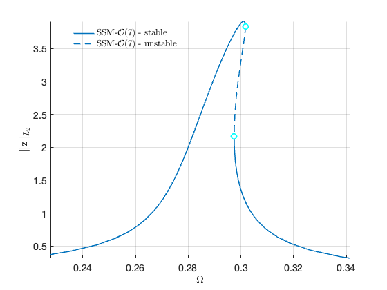
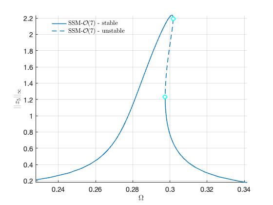
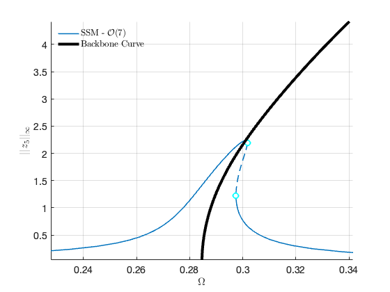
Now we proceed to plot the backbone curve on top of the forced response, for visualising the relation between the two quantities.

hold on;
plot([BB.Omega],[BB.Aout], 'Color' , 'black', 'LineWidth',4)
legend('$$\textrm{SSM - }\mathcal{O}(7)$$','','Backbone Curve','Interpreter','latex')

Computing backbone curves

Contents

SSM Computation

Example

Linear Modal analysis and SSM setup

Setup SSM computation