COHOMOLOGICAL_SOLUTION

Contents

function [W_0i, R_0i,multi_input] = cohomological_solution(obj, i,  W_0, R_0,multi_input,DStype)
        

This function computes the solution of the invariance equation at order i. The function computes the SSM where we solve the invariance equation

$\mathbf{B}D\mathbf{S}\mathbf{R}=\mathbf{A}\mathbf{S}+\mathbf{F}\circ\mathbf{S}$

of the dynamical system

$\mathbf{B}\dot{\mathbf{z}} = \mathbf{A}\mathbf{z} + \mathbf{F(\mathbf{z})}$ .

Tensor based computation

The SSM is expressed in terms of the expansion

$\mathbf{S}(\mathbf{p})=\sum_{i=1}^{\Gamma_{S}}\mathbf{S}_{i}\mathbf{p}^{\otimes i},$

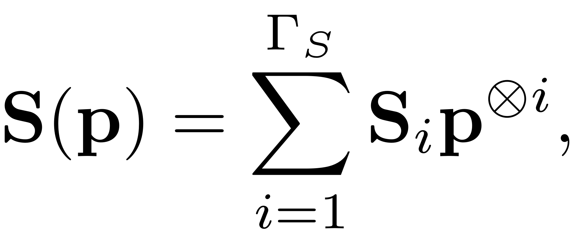
where $\mathbf{p}\in\mathbf{C}^m$ are parameterization coordinates of the $m$ -dimensional SSM.

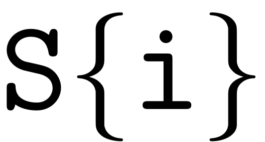The coefficients at different orders are collected in a cell array $\texttt{S}$ , where $\texttt{S\{i\}}$ gives the coefficients at order $\texttt{i}$ , i.e. $\mathbf{S}_{i}$ . These are obtained by solving for $\mathbf{S}_{i}$ in the following equation

$\mathbf{B}\mathbf{S}_{i}\mathbf{\Lambda}_{\mathcal{M},i}-\mathbf{A}\mathbf{S}_{i}=\underbrace{\sum_{j=2}^{i}\mathbf{F}_{j}\sum_{|\mathbf{p}|=i}\mathbf{S}_{p_{1}}\otimes\dots\otimes\mathbf{S}_{p_{j}}-\mathbf{B}\sum_{j=2}^{i-1}\mathbf{S}_{j}\sum_{|\mathbf{p}|=1}\mathbf{R}_{i+1-j}^{p_{1}}\otimes\dots\otimes\mathbf{R}_{i+1-j}^{p_{j}}}_{\mathbf{L}_{i}}-\mathbf{B}\mathbf{S}_{1}\mathbf{R}_{i}$

where

$\mathbf{\Lambda}_{\mathcal{M},i}:=\sum_{|\mathbf{p}|=1}\mathbf{\Lambda}_{\mathcal{M}}^{p_{1}}\otimes\dots\otimes\mathbf{\Lambda}_{\mathcal{M}}^{p_{i}}$

and $\mathbf{\Lambda}_{\mathcal{M}}$ is a diagonal ( $m\times m$ ) matrix containing the eigenvalues of the master modal subspace $\mathcal{M}$ . The above equation in the vectorized notation is given by

$\underbrace{\left[\left(\mathbf{\Lambda}_{\mathcal{M},i}^{\top}\otimes\mathbf{B}\right)-\left(\mathbf{I}_{m^{i}}\otimes\mathbf{A}\right)\right]}_{{\mathcal{C}}_{i}}\textrm{vec}\left(\mathbf{S}_{i}\right)=\textrm{vec}\left(\mathbf{L}_{i}\right)-\left(\mathbf{I}_{m^{i}}\otimes\mathbf{B}\mathbf{S}_{1}\right)\textrm{vec}\left(\mathbf{R}_{i}\right)$

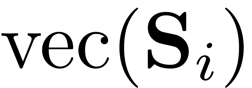Here $\textrm{vec}(\mathbf{S}_{i})$ just stands for the vectorization operator in MATLAB obtained by the command $\texttt{S\{i\}(:)}$ .

switch obj.Options.notation
    case 'tensor'
        

        Lambda_M = obj.E.spectrum;
        A = obj.System.A; % A matrix
        B = obj.System.B; % B matrix
        W_M = obj.E.adjointBasis; % Right eigenvectors of the modal subspace
        V_M = obj.E.basis; % Left eigenvectors of the modal subspace
        N = obj.dimSystem; % Full system dimensionality in first-order form
        F = obj.System.F; % Full system Nonlinearity coefficients at different orders
        m = length(Lambda_M); % dim(M): M is the master modal subspace
        N_i = N*m^i; % number of unknown SSM coefficients in the tensor notation at order i
        ref = min(abs(Lambda_M));
        if ref<1e-10; ref = max(abs(Lambda_M)); end
        abstol = obj.Options.reltol * ref;
        

Assemble the coefficient matrix of SSM

Obtaining $\mathbf{\Lambda}_{\mathcal{M},i}:=\sum_{|\mathbf{p}|=1}\mathbf{\Lambda}_{\mathcal{M}}^{p_{1}}\otimes\dots\otimes\mathbf{\Lambda}_{\mathcal{M}}^{p_{i}}$

We assemble it as

$\mathbf{\Lambda}_{\mathcal{M},i}=\sum_{j=1}^{m}\mathbf{I}_{m}\otimes\dots\otimes\mathbf{I}_m\otimes\mathbf{\Lambda}_{\mathcal{M}}\otimes\mathbf{I}_m\otimes\dots\otimes\mathbf{I}_{m}\,,$

where each term is a kronecker product of $m$ matrices and $\mathbf{\Lambda}_{\mathcal{M}}$ occurs at the $j$ -th location.

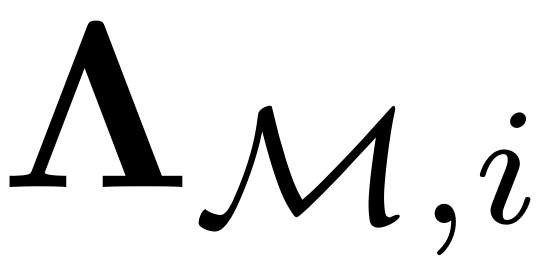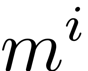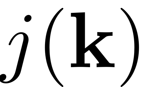We can show that the diagonal matrix $\mathbf{\Lambda}_{\mathcal{M},i}$ contains $m^i$ non-zero elements $(\mathbf{\Lambda}_{\mathcal{M},i})_{j(\mathbf{k})} = \lambda_{k_1}+\dots+ \lambda_{k_i},\quad \mathbf{k}\in\mathbf{N}^i$ and ${j(\mathbf{k})}$ represents the lexicographical bijective indexing of $i$ -tuples taking values from $1,\dots,m$ and is given by the combinator function.

        disp(['Computing autonomous whisker at order ' num2str(i)])
        combinations = combinator(m,i,'p','r');
        Lambda_Mi = sum(Lambda_M(combinations),2);
        

Spectrum of $\mathcal{C}_i:=\left[\left(\mathbf{\Lambda}_{\mathcal{M},i}^{\top}\otimes\mathbf{B}\right)-\left(\mathbf{I}_{m^{i}}\otimes\mathbf{A}\right)\right]$

The matrix that needs to be inverted for solving the coefficients at the $i$ -th order is given by

$\mathcal{C}_i:=\left[\left(\mathbf{\Lambda}_{\mathcal{M},i}^{\top}\otimes\mathbf{B}\right)-\left(\mathbf{I}_{m^{i}}\otimes\mathbf{A}\right)\right]$

Assemble RHS

$\mathbf{L}_i =\sum_{j=2}^{l}\mathbf{F}_{j}\sum_{|\mathbf{p}|=i}\mathbf{S}_{p_{1}}\otimes\dots\otimes\mathbf{S}_{p_{j}}-\mathbf{B}\sum_{j=2}^{i-1}\mathbf{S}_{j}\sum_{|\mathbf{p}|=1}\mathbf{R}_{i+1-j}^{p_{1}}\otimes\dots\otimes\mathbf{R}_{i+1-j}^{p_{j}}$

where $l=\min(i,\Gamma_F)$ since we need to compute the summation at most up to the order of the nonlinearity in $\mathbf{F}$ .

        SIZE = [N, m*ones(1,i)];
        FS = sptensor(SIZE);
        

First term

        l = min(i,length(F));
        for j = 2:l           % Outer for loop can be parallelized - l cores
            % find values for j positive numbers summing up to i
            P = nsumk(j,i,'positive');
            FS = FS + tensor_composition(F{j},W_0,P,SIZE);
        end
        

Second term

        SR = sptensor(SIZE);
        % R_0i = R_0(i:-1:2); % used for parfor
        for j = 2:i-1         % Outer for loop can be parallelized - i-1 cores
            P = ones(j,j) + eye(j,j);
            R_j = {sptensor(speye(m,m)),R_0{i+1-j}};
            % R_j = {sptensor(speye(m,m)),R_0i{j}}; % used for parfor
            SR = SR + tensor_composition(W_0{j},R_j,P,SIZE);
        end
        if m==1 % tensor_toolbox has issues
            if ~isempty(FS.vals)
                FS = sparse(FS.subs(:,1), FS.subs(:,2), FS.vals, N_i, 1);
            else
                FS = sparse(N_i,1);
            end

            if ~isempty(SR.vals)
                SR = sparse(SR.subs(:,1), SR.subs(:,2), SR.vals, N_i, 1);
            else
                SR = sparse(N_i,1);
            end
            L_i = FS - B*SR;

        else
        

            L_i = FS - ttm(SR,B,1);
        

Convert 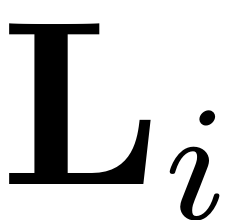$\mathbf{L}_i$ object to sparse vector.

            L_i = sptenmat(permute(L_i,[1, ndims(L_i):-1:2]), 1:ndims(L_i));
            if isempty(L_i.vals)
                L_i = sparse(N_i,1);
            else
                L_i = sparse(L_i.subs(:,1),L_i.subs(:,2),L_i.vals,N_i,1);
            end
            L_i = reshape(L_i,N,[]);
        

        end
        

Solving for SSM coefficients and Reduced dynamics

${{\mathcal{C}}_{i}}~\textrm{vec}\left(\mathbf{S}_{i}\right)=\textrm{vec}\left(\mathbf{L}_{i}\right)-\underbrace{\left(\mathbf{I}_{m^{i}}\otimes\mathbf{B}\mathbf{S}_{1}\right)}_{{\mathcal{D}}_{i}}\textrm{vec}\left(\mathbf{R}_{i}\right)$

        W_0i = zeros(N,m^i); % generally dense
        R_0i = sparse(m,m^i);

        nRes = 0;
        paramStyle = obj.Options.paramStyle;
        parfor l = 1:m^i
        

            lambda_l = Lambda_Mi(l);
            C_l = lambda_l * B - A;
            L_il = L_i(:,l);
        

Checking for near-inner resonances.

            J = find(abs(lambda_l - Lambda_M)<abstol);

            if ~isempty(J)
                switch paramStyle
                    case 'normalform'
        

Choosing reduced dynamics using (near-)kernel of $\mathcal{C}_i$ .

                        R_0il = zeros(m,1); % for slicing use
                        for j = J
                            w_j = W_M(:,j);
                            % R_0i(j,l) = w_j'*L_il;
                            R_0il(j) = w_j'*L_il;
                        end
                        R_0i(:,l) = R_0il;
        

                    case 'graph'
                        R_0i(:,l) = W_M'*L_il;
                end
                b_l = L_il - B * V_M * R_0i(:,l);
            else
                b_l = L_il;
            end
            nRes = nRes + numel(J);
        

Obtaining minimum-norm solution for 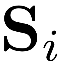$\mathbf{S}_i$ using $\texttt{lsqminnorm}$ which performs a complete orthogonal decomposition and is better suited for sparse matrices as opposed to the Moore-Penrose pseudo-inverse ( $\texttt{pinv}$ ). We would like to use better iterative procedures moving forward, currently lsqlin is not suited for complex data entries.

            W_0i(:,l) = solveinveq(C_l,b_l,obj.Options.solver);
        

        end
        disp([num2str(nRes) ' (near) inner resonance(s) detected at order ' num2str(i)])

        W_0i = reshape(sptensor(W_0i(:)), [N, m*ones(1,i)]);
        R_0i = reshape(sptensor(R_0i(:)), [m, m*ones(1,i)]);
        W_0i = permute(W_0i,[1, ndims(W_0i):-1:2]);
        R_0i = permute(R_0i,[1, ndims(R_0i):-1:2]);
        

    case 'multiindex'
        

        k   = i;                     % order of computation
        N   = obj.dimSystem;         % Phase space dimension
        l   = numel(obj.E.spectrum); % Manifold dimension

        % ################################################################
        %      Setup data structs for passing arguments into functions

        % system parameters independent of multi- index ordering
        sys.l      = l;
        sys.N      = N;
        sys.V_M    = obj.E.basis;
        sys.W_M    = obj.E.adjointBasis;
        sys.solver = obj.Options.solver;
        sys.reltol = obj.Options.reltol;
        sys.DStype = obj.System.Options.DStype;

        % data containing information about nonlinearity
        [NL,nl_data] = NLdata(obj);
        sys.nl_order = nl_data.order;
        sys.nl_input_dim  = nl_data.nl_input_dim;

        % ################################################################
        % ---- variables that depend on multi-index ordering ----

        K        = flip(sortrows(nsumk(l,k,'nonnegative')).',2);
        z_k      = data.Z_cci(k);                % number of multi_indices

        if strcmp(sys.DStype,'real')
            K = K(:,data.revlex2conj{k}(1:z_k)); % conjugate ordered set
            sys.revlex2conj = data.revlex2conj;  % ordering of conjugate set
            sys.Z_cci       = data.Z_cci;        % conj. center index
        end

        sys.Lambda_M_vector = data.Lambda_M_vector;
        sys.ordering        = data.ordering;
        sys.z_k             = z_k;
        sys.K               = K;
        sys.k               = k;


        % ################################################################
        % ################################################################
        %         Assemble the right hand side of the invarinace eq.

        % Mixed Terms
        WR = zeros(N,z_k);





        mix = tic;
        for m = 2:k-1
            WR = WR - coeffs_mixed_terms(k,m,W_0,R_0,sys,'aut');
        end
        mixtime = toc(mix);

        % The composition coefficients of power series
        if nl_data.intrusion
            H   = data.H;    % composition coefficients
            H_k  = coeffs_composition(W_0,H,sys);
            H{k} = H_k;
        end

        % Nonlinearity contributions to invariance equation
        Fn = zeros(N,z_k);













        nl = tic;
        switch nl_data.mode
            case 'IntrusiveF'
                sys.symmetry = obj.System.F_semi_sym; % whether function handles are symmetric
                for n = 2:min(k,nl_data.order)
                    if ~isempty(NL{n})
                        Fn  = Fn + fnl_semiIntrusive(NL{n},W_0,n,K,sys);
                    end
                end

            case 'SemiIntrusiveF'
                sys.symmetry = obj.System.F_semi_sym; % whether function handles are symmetric
                for n = 2:min(k,nl_data.order)
                    if ~isempty(NL{n})
                        Fn  = Fn + fnl_semiIntrusive(NL{n},W_0,n,K,sys);
                    end
                end

            case 'NonIntrusiveF'
                for n = 2:3
                    if ~isempty(NL)
                        Fn  = Fn + fnl_nonIntrusive(NL,W_0,n,K,sys);
                    end
                end





        end













        nltime = toc(nl);
        % saving memory
        if ~any(Fn)
            Fn = sparse(N,z_k);
        end

        if ~any(WR)
            WR = sparse(N,z_k);
        end


        % ################################################################
        %  ################################################################
        %      Solving invariance equation and determine reduced dynamics






        %  ################################################################
        %       Computation for first order dynamical systems









        if strcmp(obj.Options.COMPtype,'first')

            A   = obj.System.A; % A matrix
            B   = obj.System.B; % B matrix



            RHS = B*WR + Fn;
            RHS = reshape(RHS,N*z_k,1);







            invtic = tic;
            [R_0i,W_0i,eqtime,rdtime] = Aut_1stOrder_SSM(RHS, sys,A,B);
            invtime = toc(invtic);

        % #################################################################
        %       Computation for second order dynamica lsystems
        else
            Mass      = obj.System.M;
            Damp      = obj.System.C;
            Stiff     = obj.System.K;

            invtic = tic;
            [R_0i,W_0i,eqtime,rdtime] = Aut_2ndOrder_SSM(WR,Fn,sys,Mass,Damp,Stiff);
            invtime = toc(invtic);
        end
        

pass on composition coefficients

        if nl_data.intrusion
            H_k(:,:,1) = W_0i;
            H{k}       = H_k;
            data.H = H;
        end

        obj.solInfo.mixTime(i)= mixtime;
        obj.solInfo.invTime(i) = invtime;
        obj.solInfo.eqTime(i) = eqtime;
        obj.solInfo.nlTime(i) = nltime;
        obj.solInfo.rdTime(i) = rdtime;
        

end
% estime memory consumption from all variables in the current workspace
obj.solInfo.memoryEstimate(i) = monitor_memory('caller');
        

end

function [NL,data] = NLdata(obj)
        

% NL   - contains nonlinearity ot potential
% data - contains information about NL





data.intrusion = false;
data.nl_input_dim   = [];

intr_opt = obj.System.Options.Intrusion;
        

Assert that valid option has been chosen for computation

assert(strcmp(intr_opt ,'semi') || strcmp(intr_opt,'none')|| strcmp(intr_opt,'full'),...
    'Intrusion options are: full, none, semi')




switch obj.System.Options.Intrusion
    case 'semi'
        data.mode = 'SemiIntrusiveF';
        % Full system nonlinearity handles at different orders
        NL   = obj.System.F_semi;








        % check input dimensionality of function handles
        data.nl_input_dim = obj.System.nl_input_dim;


    case 'none'
        data.mode = 'NonIntrusiveF';
        % Full system nonlinearity handles at different orders
        NL   = obj.System.F_non;

        % check input dimensionality of function handles
        data.nl_input_dim = obj.System.nl_input_dim;

    case 'full'
        data.intrusion = true;
        data.mode = 'IntrusiveF';
        % Full system nonlinearity coefficients at different orders

        switch obj.System.order
            case  1
                for j = 2:numel(obj.System.F)
                    if ~isempty(obj.System.F{j}) && nnz(obj.System.F{j})>0
                        F{j} = @(input) double(ttv( obj.System.F{j},input,2:j+1));
                    end
                end
            case 2
                for j = 1:numel(obj.System.fnl)
                    if ~isempty(obj.System.fnl{j}) && nnz(obj.System.fnl{j})>0
                        F{j+1} = @(input) [-double(ttv( obj.System.fnl{j},input,2:j+2)) ; sparse(obj.System.n,1)];
                    end
                end
        end

        data.nl_input_dim = obj.System.nl_input_dim;
        NL   = F;
end
data.order = numel(NL);
        

end
        

Published with MATLAB® R2023a