Setting up Dynamical Systems
Contents
In an initial step the order of the dynamical system has to be specified. This has to be done when initialisng the dynamical system via
DS = DynamicalSystem(order);
Depending on the dynamical system which is to be analysed, the following procedures have to be followed.
Setting up a Second Order Dynamical System
In this section we explain how DynamicalSystem constructs a dynamical system object in second order form which is given as:
 - Second order
The linear system matrices can be set via the set method of the class as
set(DS,'M',M,'C',C,'K',K);
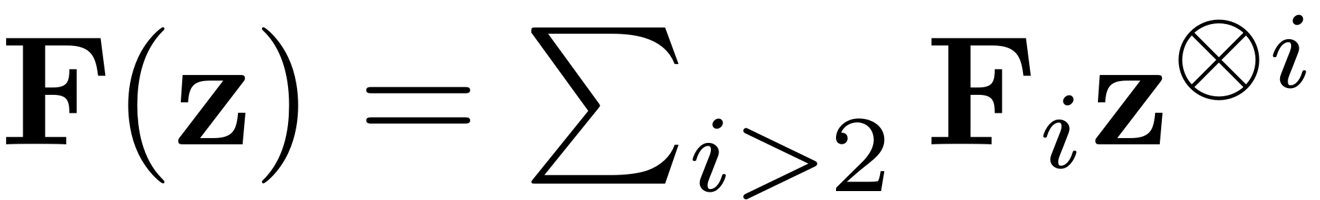
 is a nonlinear polynomial function of degree two or higher an can
also be set with the set method as.
is a nonlinear polynomial function of degree two or higher an can
also be set with the set method as.
set(DS,'fnl',fnl);
This nonlinear force may be prepared in one of the following ways:
Using tensor format:
In tensor notation the second order nonlinear internal forces are expanded as
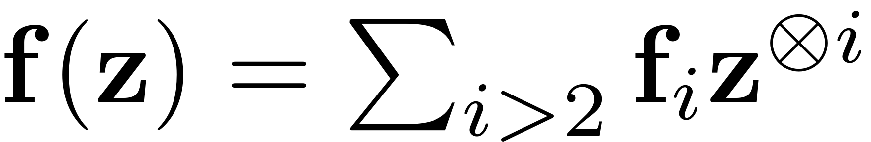
The order i nonlinearity is thus represented by a
 dimensional tensor
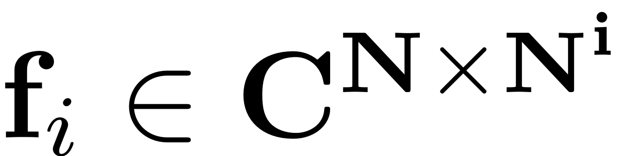 . For implementation it is represented by a multidimensional array
of dimension
. These arrays are stored in a cell array. So in this case one might
obtain the order i nonlinearity as
. For implementation it is represented by a multidimensional array
of dimension
. These arrays are stored in a cell array. So in this case one might
obtain the order i nonlinearity as
fi = f{i}
Here
 is a polynomial function of degree two or higher, which is stored as
a cell array such that
is a polynomial function of degree two or higher, which is stored as
a cell array such that
 corresponds to polynomials of degree k+1.
is given by a tensor of order k+2, where the first mode corresponds
to indices for the force vector.
corresponds to polynomials of degree k+1.
is given by a tensor of order k+2, where the first mode corresponds
to indices for the force vector.
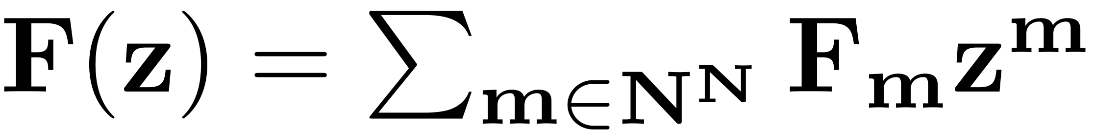
Using multi-index format: In multi-index notation the second order nonlinear internal forces are expanded as
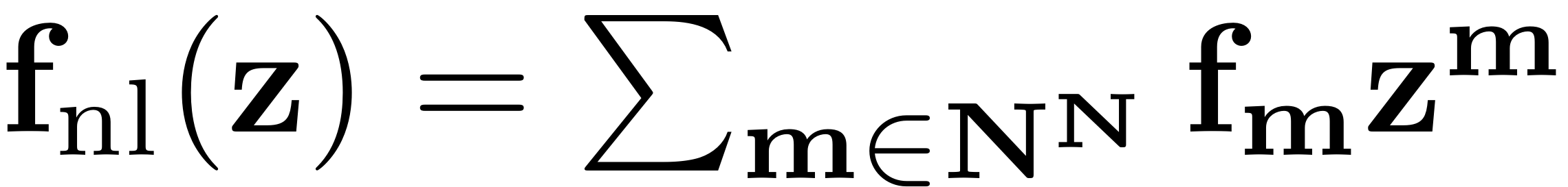
The variate monomials in this expansion are written as
 . The nonlinearity in this case is stored in a struct array with
fields that characterise its coefficients and the corresponding
multi-indices. Thus the relevant quantities are stored
. The nonlinearity in this case is stored in a struct array with
fields that characterise its coefficients and the corresponding
multi-indices. Thus the relevant quantities are stored
fm = f(m_abs).coeffs
fm  = f(m_abs).ind
This extracts all coefficients of the Taylor expansion and the
corresponding order
 multi-indices m. So
 is a
is a
 and
and
 is a
dimensional array, where
is a
dimensional array, where
 denotes the number of unique multi-indices at order
.
denotes the number of unique multi-indices at order
.
In case of velocity-independent internal forces, the tensors and multi-indices are of lower dimensionality respectively, as they only require half the input variables to describe the action of the forces.
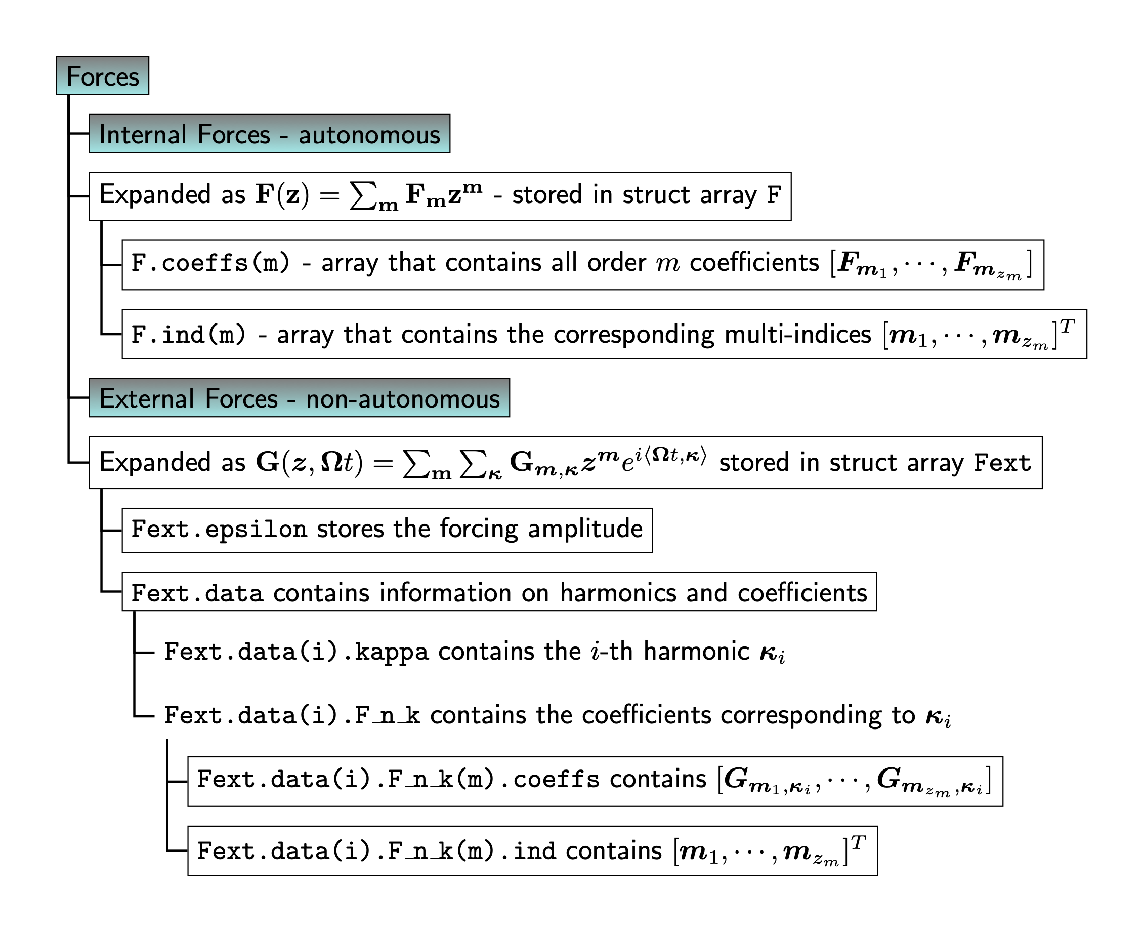
Second order external excitation
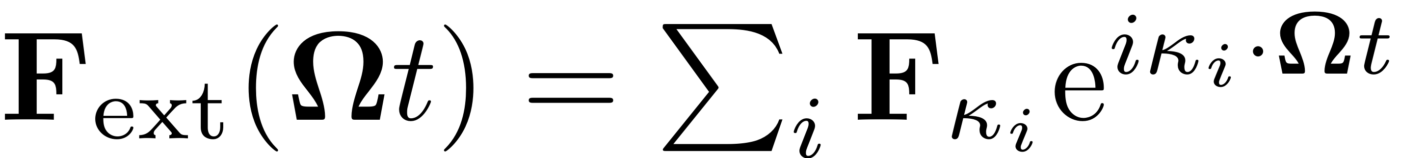
The external force is provided as a Fourier Expansion in terms of the relevant harmonics.
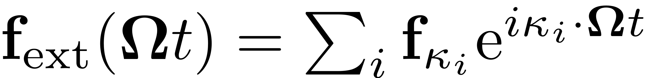
Furthermore the forcing frequency is given by a frequency vector. This force may be input to the dynamical system in various formats:
Format 1: As a struct array
fext.epsilon = epsilon
fext.data    = data
where
 is a struct array with entries
data(i).kappa = kappa_i
data(i).coeffs = f_kappa_i
In this case it is passed to the DS object as
DS.add_forcing(fext)
Format 2: With harmonics and coefficients
If only a single harmonic is used for a periodic excitation, the
harmonics
 and the coefficients
 can be input manually as
coeffs = [f_kappa_1, f_kappa_2]
Kappas = [kappa_1, kappa_2]
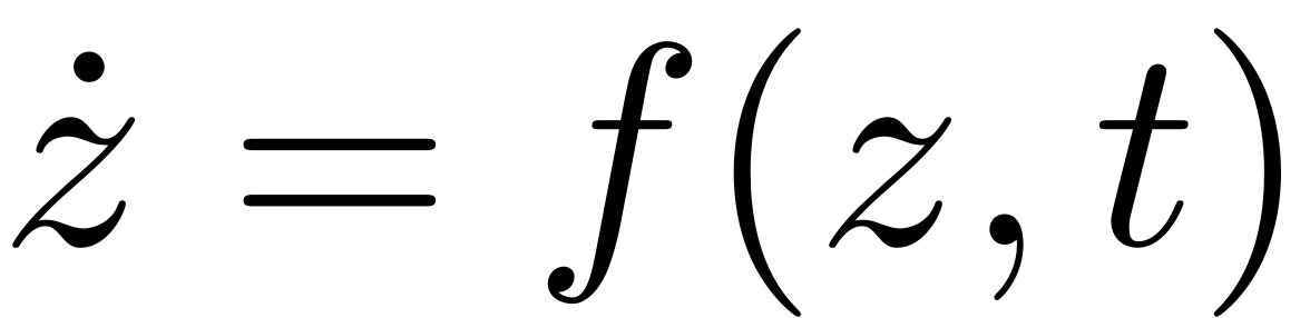
The second order form is converted into the first order form with
![$$ \mathbf{z}=\left[\begin{array}{c}\mathbf{x}\\\dot{\mathbf{x}}\end{array}\right],
\quad\mathbf{A}=\left[\begin{array}{cc}-\mathbf{K} & \mathbf{0}\\\mathbf{0} & \mathbf{M}\end{array}\right],
\mathbf{B}=\left[\begin{array}{cc}\mathbf{C} & \mathbf{M}\\\mathbf{M} & \mathbf{0}\end{array}\right],
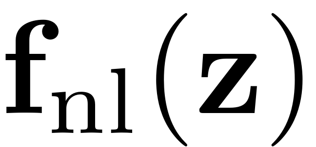
\quad\quad\mathbf{F}(\mathbf{z})=\left[\begin{array}{c}-\mathbf{f}_{\textrm{nl}}(\mathbf{x},\dot{\mathbf{x}})\\\mathbf{0}\end{array}\right],
\quad\mathbf{F}_\textrm{ext}(\mathbf{z},\mathbf{\Omega} t) =\left[\begin{array}{c}\mathbf{f}_{\textrm{ext}}(\mathbf{\Omega} t)\\ \mathbf{0} \end{array}\right] $$](SetupDS_Explanation_eq14245467934836547411-Rescaled.png)
Setting up a First Order Dynamical System
In this section we explain how the
 class constructs a dynamical system object in first order form which
is given as:
class constructs a dynamical system object in first order form which
is given as:
 The linear system matrices can be set via the set method of the
class as
The linear system matrices can be set via the set method of the
class as
set(DS,'A',A,'B',B);
 is a nonlinear polynomial function of degree two or higher an can
also be set with the set method as.
is a nonlinear polynomial function of degree two or higher an can
also be set with the set method as.
set(DS,'F',F);
This nonlinear force may be prepared in one of the following ways:
Using tensor format:
In tensor notation the first order nonlinear internal forces are expanded as
The order i nonlinearity is thus represented by a
dimensional tensor
 . For implementation it is represented by a multidimensional array
of dimension
. These arrays are stored in a cell array. So in this case one might
obtain the order i nonlinearity as
. For implementation it is represented by a multidimensional array
of dimension
. These arrays are stored in a cell array. So in this case one might
obtain the order i nonlinearity as
Fi = F{i}
Using multi-index format: In multi-index notation the first order nonlinear internal forces are expanded as
The variate monomials in this expansion are written as
. The nonlinearity in this case is stored in a struct array with
fields that characterise its coefficients and the corresponding
multi-indices. Thus the relevant quantities are stored
Fm = F(m_abs).coeffs
m  = F(m_abs).ind
This extracts all coefficients of the Taylor expansion and the
corresponding order
multi-indices m. So
is a
 and
is a
dimensional array, where
and
is a
dimensional array, where
 denotes the number of unique multi-indices at order
.
denotes the number of unique multi-indices at order
.
First order external excitation
The external force is provided as a Fourier Expansion in terms of the relevant harmonics.
Furthermore the forcing frequency is given by a frequency vector. This force may be input to the dynamical system in various formats:
Format 1: As a struct array
Fext.epsilon = epsilon
Fext.data    = data
where
is a struct array with entries
data(i).kappa = kappa_i
data(i).coeffs = F_kappa_i
In this case it is passed to the DS object as
DS.add_forcing(Fext)
Format 2: With harmonics and coefficients
If only a single harmonic is used for a periodic excitation, the
harmonics
and the coefficients
 can be input manually as
coeffs = [F_kappa_1, F_kappa_2]
Kappas = [kappa_1, kappa_2]
In general, the nonlinear and external forces are stored as follows:
Specifications
Several options can be passed to the dynamical system class, to further specify characteristics of the underlying system, as well as how it is supposed to be handled computationally. In the following they are presented with their default values. If a system with non default parameters is treated, these have to be adapted.
set(DS.Options,'Nmax',6);               % Maximal sytem size for which the full spectrum is computed
set(DS.Options,'Emax',10);              % Maximal number of Eigenvalues and -vectors that are computed if system size is larger than Nmax
set(DS.Options,'notation','multiindex');% Notation in which nonlinear forces are to be handled, can be 'multiindex' or 'tensor'
set(DS.Options,'RayleighDamping',true); % Whether the underlying damping model is of Rayleigh Type
set(DS.Options,'BaseExcitation',false); % Whether the external force arises due to an excitation of the base which leads to a frequency dependent forcing amplitude.
set(DS.Options,'DStype','real');        % To determine whether dynamical system possesses any complex valued quantities.
set(DS.Options,'outDOF',[]);            % For which DOF of the full system the relevant quantities should be explicitly displayed and stored.
set(DS.Options,'HarmonicForce',true);   % To determine whether time dependence of the external forcing is harmonic or not
set(DS.Options,'lambdaThreshold',1e16); % Threshold beyond which stiff eigenmodes will be removed
set(DS.Options,'sigma',0);              % value around which eigenvalues are computed. Is set to zero by default which corresponds to the 'smallestabs' setting in the built in eigs function.
set(DS.Options,'RemoveZeros',true);     % Remove eigenvalues with zero real part from the spectrum. Relevant for the computation of center manifolds and in parameter dependent SSMs.
Methods
The first and crucial method which is provided for the DS class is
the
 method, which solves specified bits of the eigenvalue problem for
the linear truncation of the dynamical system that is input. It is
invoked via
method, which solves specified bits of the eigenvalue problem for
the linear truncation of the dynamical system that is input. It is
invoked via
[V,D,W] = DS.linear_spectral_analysis();
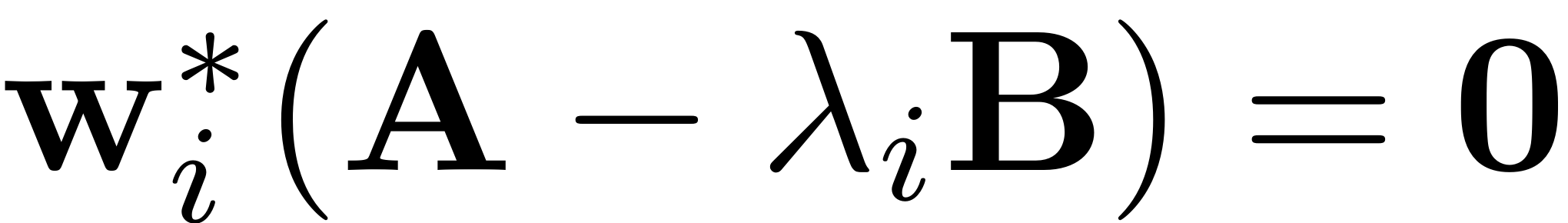
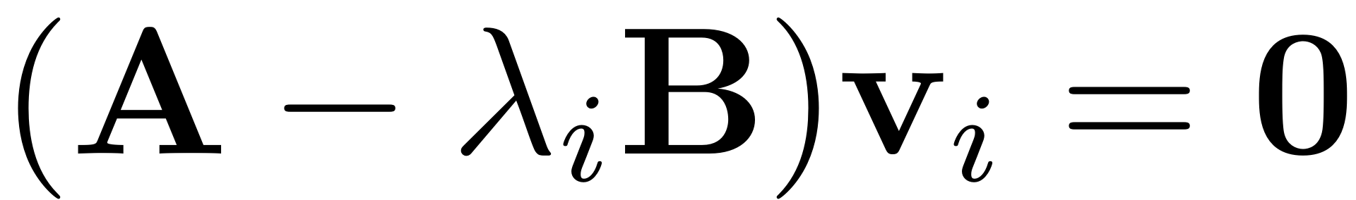
When run, it outputs the three arguments the left and right eigenvectors and the eigenvalues of the eigenproblems
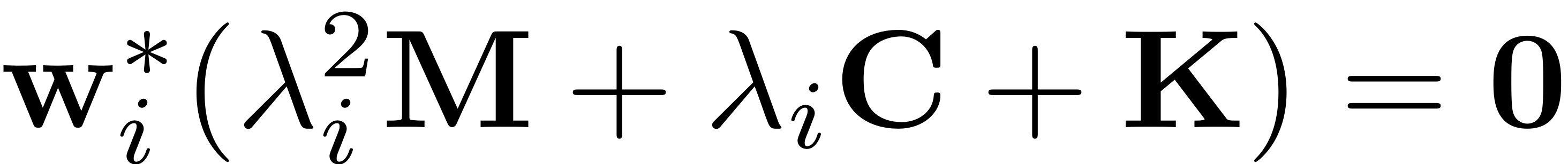
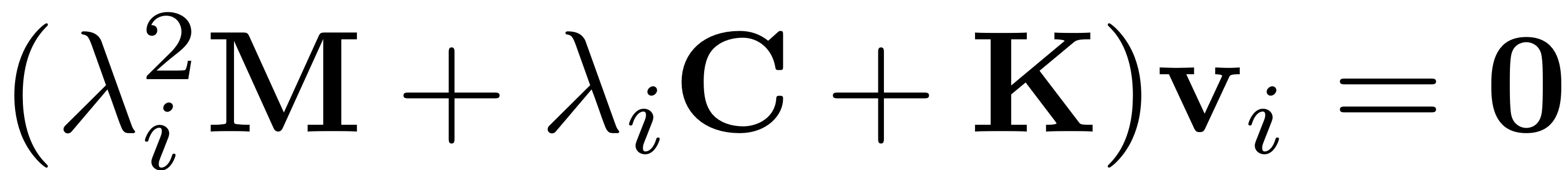
or
Furthermore it sets up an internal data structure with fields that contain the essential information about the truncated spectrum of the dynamical system which are used for invariant manifold computations.
For the evaluation of the nonlinear internal and the external forces the following functions are provided.
fnl = DS.compute_fnl(x,xd);
Fnl = DS.evaluate_Fnl(z);
fext = DS.compute_fext(t,x);
Fext = DS.evaluate_Fext(t,z);
These are also used for the construction of the governing ODE
 which is evaluated via
f = DS.odefun(t,z);
Further functionalities which are provided for this class include the evaluation of the Jacobians of the nonlinear internal forces via
dfnldx = DS.compute_dfnldx(x,xd);
dfnldxd = DS.compute_dfnldxd(x,xd);
and the residual that may be used for the integration of ODEs,
[ r, drdqdd,drdqd,drdq, c0] = DS.residual(q, qd, qdd, t);