Prismatic Beam Stretching
We consider a clamped-pinned beam. With such a boundary condition, the first two modes have near 1:3 internal resonance as follows
with .
Nayfeh [1] inverstigated the forcec response of such a system under external harmonic response. Specifically, modal expansion (with linear modes) is used to transfer PDEs to a set of ODEs
Then multiple scale perturbation method is used to study the forced response curve. Interestingly, when the excitation frequency is around the second natural frequency, there exits solution branches where the amplitude of the first mode dominiates the system response. Here we use SSM reduction to study such a system.
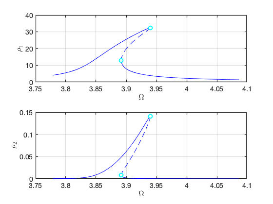
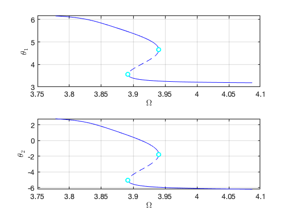
Here we will use the SSM-ep toolbox to calculate the forced response curve. The reader is encouraged to use extract_FRC routine to repeat the analysis.
[1] Nayfeh, A. H., Mook, D. T., & Sridhar, S. (1974). Nonlinear analysis of the forced response of structural elements. The Journal of the Acoustical Society of America, 55(2), 281-291.
Contents
Setup Dynamical System
clear all;
epsilon = 1e-4;
c  = 100;
f = 5/epsilon;
n = 10;               % number of modes
Fext = zeros(n,1);    % excitation at modal coordinate
Fext(1) = f;
[mass,damp,stiff,fnl,fext] = build_model(c,Fext,epsilon,n);
Getting nonlinearity coefficients
Loaded coefficients from storage
Create the dynamical system
order = 2;
DS = DynamicalSystem(order);
set(DS,'M',mass,'C',damp,'K',stiff,'fnl',fnl);
set(DS.Options,'Emax',5,'Nmax',10,'notation','multiindex')
% Forcing
kappas = [-1; 1];
coeffs = [fext fext]/2;
DS.add_forcing(coeffs, kappas);
Linear Modal analysis
[V,D,W] = DS.linear_spectral_analysis();
Due to high-dimensionality, we compute only the first 5 eigenvalues with the smallest magnitude. These would also be used to compute the spectral quotients
Assuming a proportional damping hypthesis with symmetric matrices
modal damping ratio for 1 mode is 2.593810e-03
modal damping ratio for 2 mode is 8.004681e-04
modal damping ratio for 3 mode is 3.837148e-04
modal damping ratio for 4 mode is 2.243713e-04
modal damping ratio for 5 mode is 1.470421e-04

 The first 10 nonzero eigenvalues are given as
  -0.0100 + 3.8553i
  -0.0100 - 3.8553i
  -0.0100 +12.4927i
  -0.0100 -12.4927i
  -0.0100 +26.0610i
  -0.0100 -26.0610i
  -0.0100 +44.5690i
  -0.0100 -44.5690i
  -0.0100 +68.0077i
  -0.0100 -68.0077i
Choose Master subspace (perform resonance analysis)
Due to the 1:3 internal resonance, we take the first two complex conjugate pairs of modes as the spectral subspace to SSM. So we hvae resonant_modes = [1 2 3 4].
S = SSM(DS);
set(S.Options, 'reltol', 1,'notation','multiindex');
resonant_modes = [1 2 3 4];
order = 3;
outdof = [1 2];
Primary resonance of the first mode
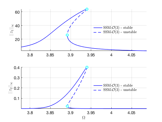
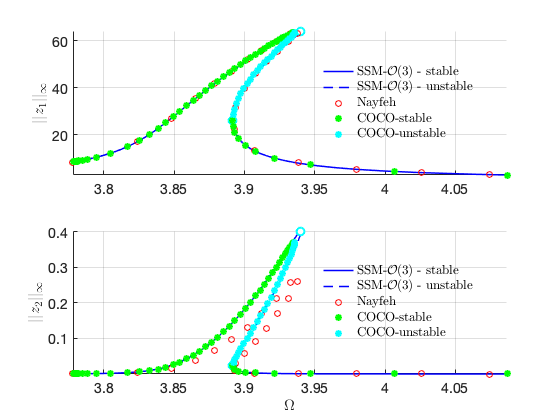
We first consider the case that . Although only the first mode is excited externally (), the response of the second mode is nontrivial due to the modal interactions.
freqrange = [0.98 1.06]*imag(D(1));
set(S.FRCOptions, 'nCycle',500, 'initialSolver', 'forward');
set(S.contOptions, 'PtMX', 300, 'h_max', 0.5);
set(S.FRCOptions, 'omegaSampStyle', 'cocoBD');
start = tic;
FRC_ep1 = S.SSM_isol2ep('isol',resonant_modes, order, [1 3], 'freq', freqrange,outdof);
timings.FRC_ep1 = toc(start)
The master subspace contains the following eigenvalues

lambda1 == - 0.01 + 3.8553i

lambda2 == (-0.01) - 3.8553i

lambda3 == - 0.01 + 12.4927i

lambda4 == (-0.01) - 12.4927i

sigma_out = 1
sigma_in = 1
Manifold computation time at order 2 = 00:00:00
Estimated memory usage at order  2 = 7.03E-02 MB
Manifold computation time at order 3 = 00:00:00
Estimated memory usage at order  3 = 1.03E-01 MB

 Run='isol.ep': Continue equilibria along primary branch.

    STEP   DAMPING               NORMS              COMPUTATION TIMES
  IT SIT     GAMMA     ||d||     ||f||     ||U||   F(x)  DF(x)  SOLVE
   0                          6.25e-01  2.38e+01    0.0    0.0    0.0
   1   1  5.09e-01  1.26e+00  1.04e-01  2.38e+01    0.0    0.0    0.0
   2   1  1.00e+00  3.85e-01  1.81e-02  2.38e+01    0.0    0.0    0.0
   3   1  1.00e+00  8.11e-03  3.47e-04  2.38e+01    0.0    0.0    0.0
   4   1  1.00e+00  7.84e-06  1.28e-07  2.38e+01    0.0    0.0    0.0
   5   1  1.00e+00  3.01e-09  1.80e-14  2.38e+01    0.0    0.1    0.0

 STEP      TIME        ||U||  LABEL  TYPE            om         rho1         rho2          th1          th2          eps
    0  00:00:00   2.3797e+01      1  EP      3.8551e+00   1.5213e+01   1.1521e-02   5.7948e+00   1.6658e+00   1.0000e+00
   10  00:00:01   2.0250e+01      2          3.8431e+00   1.2295e+01   5.8889e-03   5.8943e+00   1.9645e+00   1.0000e+00
   20  00:00:01   1.6348e+01      3          3.8260e+00   8.7778e+00   2.0455e-03   6.0090e+00   2.3093e+00   1.0000e+00
   30  00:00:02   1.3193e+01      4          3.7967e+00   5.2600e+00   4.0649e-04   6.1202e+00   2.6437e+00   1.0000e+00
   34  00:00:02   1.2414e+01      5  EP      3.7782e+00   4.0992e+00   1.8330e-04   6.1564e+00   2.7527e+00   1.0000e+00

 STEP      TIME        ||U||  LABEL  TYPE            om         rho1         rho2          th1          th2          eps
    0  00:00:02   2.3797e+01      6  EP      3.8551e+00   1.5213e+01   1.1521e-02   5.7948e+00   1.6658e+00   1.0000e+00
   10  00:00:02   2.7507e+01      7          3.8670e+00   1.8129e+01   2.0117e-02   5.6898e+00   1.3506e+00   1.0000e+00
   20  00:00:03   3.2108e+01      8          3.8819e+00   2.1638e+01   3.5585e-02   5.5525e+00   9.3816e-01   1.0000e+00
   30  00:00:03   3.6796e+01      9          3.8981e+00   2.5138e+01   5.8302e-02   5.3959e+00   4.6782e-01   1.0000e+00
   40  00:00:04   4.1520e+01     10          3.9159e+00   2.8619e+01   9.0463e-02   5.2015e+00  -1.1610e-01   1.0000e+00
   50  00:00:04   4.6135e+01     11          3.9360e+00   3.1988e+01   1.3416e-01   4.8752e+00  -1.0956e+00   1.0000e+00
   60  00:00:06   4.6725e+01     12          3.9399e+00   3.2417e+01   1.4147e-01   4.7092e+00  -1.5940e+00   1.0000e+00
   67  00:00:07   4.6646e+01     13  FP      3.9402e+00   3.2359e+01   1.4092e-01   4.6528e+00  -1.7631e+00   1.0000e+00
   67  00:00:07   4.6646e+01     14  SN      3.9402e+00   3.2359e+01   1.4092e-01   4.6528e+00  -1.7631e+00   1.0000e+00
   70  00:00:07   4.6515e+01     15          3.9401e+00   3.2264e+01   1.3969e-01   4.6153e+00  -1.8754e+00   1.0000e+00
   80  00:00:07   4.3804e+01     16          3.9330e+00   3.0287e+01   1.1356e-01   4.3478e+00  -2.6778e+00   1.0000e+00
   90  00:00:08   3.9090e+01     17          3.9201e+00   2.6830e+01   7.6346e-02   4.1163e+00  -3.3717e+00   1.0000e+00
  100  00:00:10   3.4381e+01     18          3.9088e+00   2.3336e+01   4.8855e-02   3.9451e+00  -3.8852e+00   1.0000e+00
  110  00:00:12   2.9735e+01     19          3.8999e+00   1.9831e+01   2.9372e-02   3.7997e+00  -4.3210e+00   1.0000e+00
  120  00:00:13   2.5206e+01     20          3.8939e+00   1.6320e+01   1.6181e-02   3.6691e+00  -4.7129e+00   1.0000e+00
  130  00:00:14   2.1112e+01     21  SN      3.8918e+00   1.3000e+01   8.1785e-03   3.5541e+00  -5.0576e+00   1.0000e+00
  130  00:00:14   2.1112e+01     22  FP      3.8918e+00   1.3000e+01   8.1785e-03   3.5541e+00  -5.0576e+00   1.0000e+00
  130  00:00:14   2.0879e+01     23          3.8918e+00   1.2805e+01   7.8198e-03   3.5476e+00  -5.0773e+00   1.0000e+00
  140  00:00:15   1.6920e+01     24          3.8957e+00   9.2883e+00   3.0468e-03   3.4321e+00  -5.4239e+00   1.0000e+00
  150  00:00:16   1.3661e+01     25          3.9133e+00   5.7706e+00   7.8504e-04   3.3205e+00  -5.7596e+00   1.0000e+00
  160  00:00:17   1.1750e+01     26          3.9992e+00   2.2541e+00   7.1304e-05   3.2112e+00  -6.0946e+00   1.0000e+00
  163  00:00:17   1.1636e+01     27  EP      4.0866e+00   1.4013e+00   3.6412e-05   3.1848e+00  -6.1964e+00   1.0000e+00

the forcing frequency 3.7782e+00 is nearly resonant with the eigenvalue -1.0000e-02 + i3.8553e+00
the forcing frequency 3.7803e+00 is nearly resonant with the eigenvalue -1.0000e-02 + i3.8553e+00
the forcing frequency 3.7865e+00 is nearly resonant with the eigenvalue -1.0000e-02 + i3.8553e+00
.
.
.

Verification
Load Nayfeh's solution for comparison
Nayfeh1 = load('NayfehFirstMode');
om1 = 3.8553;
omsamp = om1*(1+Nayfeh1.epsilon*Nayfeh1.SIG2);
figure(gcf); hold on
subplot(2,1,1)
plot(omsamp(1:100:end),Nayfeh1.A1(1:100:end),'ro','DisplayName','Nayfeh');
subplot(2,1,2)
plot(omsamp(1:100:end),Nayfeh1.A2(1:100:end),'ro','DisplayName','Nayfeh');
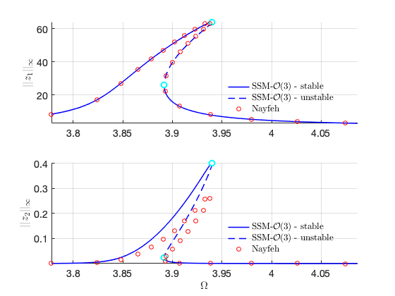
Verification using COCO The following run uses the po-toolbox of COCO to calculate the forced reponse curve of the full system with collocation methods. It can take more than 10 minutes to finish.
nCycles = 500;
coco = cocoWrapper(DS, nCycles, outdof);
set(coco.Options, 'PtMX', 1000, 'NTST',20, 'dir_name', 'bd1');
set(coco.Options, 'NAdapt', 1, 'h_max', 200, 'MaxRes', 1);
coco.initialGuess = 'linear';
start = tic;
bd1 = coco.extract_FRC(freqrange);
timings.cocoFRCbd1 = toc(start)
 Run='bd1.FRC': Continue primary family of periodic orbits.

    STEP   DAMPING               NORMS              COMPUTATION TIMES
  IT SIT     GAMMA     ||d||     ||f||     ||U||   F(x)  DF(x)  SOLVE
   0                          1.19e-01  2.33e+02    0.0    0.0    0.0
   1   1  1.00e+00  5.77e-02  1.08e-05  2.33e+02    0.0    0.6    0.2
   2   1  1.00e+00  2.21e-04  4.30e-12  2.33e+02    0.0    1.3    0.2
   3   1  1.00e+00  5.04e-10  6.73e-14  2.33e+02    0.1    1.8    0.3

 STEP      TIME        ||U||  LABEL  TYPE         omega    po.period          eps         amp1         amp2
    0  00:00:06   2.3281e+02      1  EP      3.7796e+00   1.6624e+00   1.0000e+00   8.4151e+00   6.5931e-04
    6  00:00:43   2.7340e+02      2  EP      3.7782e+00   1.6630e+00   1.0000e+00   8.2760e+00   6.2617e-04

 STEP      TIME        ||U||  LABEL  TYPE         omega    po.period          eps         amp1         amp2
    0  00:00:44   2.3281e+02      3  EP      3.7796e+00   1.6624e+00   1.0000e+00   8.4151e+00   6.5931e-04
   10  00:01:46   3.6802e+02      4          3.7952e+00   1.6556e+00   1.0000e+00   1.0351e+01   1.2579e-03
   20  00:04:23   1.4273e+03      5          3.8635e+00   1.6263e+00   1.0000e+00   3.4591e+01   5.2579e-02
   30  00:07:12   2.3385e+03      6          3.9045e+00   1.6092e+00   1.0000e+00   5.2987e+01   2.0194e-01
   40  00:10:02   2.9303e+03      7          3.9309e+00   1.5984e+00   1.0000e+00   6.2494e+01   3.4763e-01
   47  00:13:00   2.9782e+03      8  SN      3.9359e+00   1.5964e+00   1.0000e+00   6.3483e+01   3.6857e-01
   50  00:13:55   2.9190e+03      9          3.9343e+00   1.5970e+00   1.0000e+00   6.2222e+01   3.4662e-01
   60  00:17:05   2.4463e+03     10          3.9166e+00   1.6043e+00   1.0000e+00   5.2119e+01   1.9859e-01
   70  00:20:05   1.5669e+03     11          3.8940e+00   1.6135e+00   1.0000e+00   3.3211e+01   5.0002e-02
   73  00:21:47   1.2078e+03     12  SN      3.8916e+00   1.6146e+00   1.0000e+00   2.6025e+01   2.4107e-02
   80  00:23:59   2.9137e+02     13          3.9467e+00   1.5920e+00   1.0000e+00   7.0449e+00   5.6747e-04
   82  00:24:34   1.1350e+02     14  EP      4.0866e+00   1.5375e+00   1.0000e+00   2.7207e+00   7.5464e-05

Computation time:

   SSM based computation:    FRC_ep1:       34.1298
   Full system analysis:     cocoFRCbd1: 1.4807e+03
Other modes
Nonzero forcing at other modes Next we consider the case that all the ten modes are excited externally. The method of multiple scale produces the same results as before given only is involved in the secular equation for the method of multiple scale. In contrast, the SSM reduction captures well the contribution of . In particular, the method of multiple scale predictes that the for , independently of the value of .
Fext = zeros(n,1)+f;  % excitation at modal coordinate
[~,~,~,~,fext2] = build_model(c,Fext,epsilon,n);
coeffs = [fext2 fext2]/2;
DS.add_forcing(coeffs, kappas);
outdof2 = [2 3]

start = tic;
FRC_ep2 = S.SSM_isol2ep('isolAllf',resonant_modes, order, [1 3], 'freq', freqrange,outdof2);
timings.FRC_ep2 = toc(start)
Getting nonlinearity coefficients
Loaded coefficients from storage

outdof2 =

     2     3

The master subspace contains the following eigenvalues

lambda1 == - 0.01 + 3.8553i

lambda2 == (-0.01) - 3.8553i

lambda3 == - 0.01 + 12.4927i

lambda4 == (-0.01) - 12.4927i

sigma_out = 1
sigma_in = 1

Manifold computation time at order 2 = 00:00:00
Estimated memory usage at order  2 = 7.03E-02 MB
Manifold computation time at order 3 = 00:00:00
Estimated memory usage at order  3 = 1.03E-01 MB

 Run='isolAllf.ep': Continue equilibria along primary branch.

    STEP   DAMPING               NORMS              COMPUTATION TIMES
  IT SIT     GAMMA     ||d||     ||f||     ||U||   F(x)  DF(x)  SOLVE
   0                          6.25e-01  2.38e+01    0.0    0.0    0.0
   1   1  5.09e-01  1.26e+00  1.04e-01  2.38e+01    0.0    0.0    0.0
   2   1  1.00e+00  3.85e-01  1.81e-02  2.38e+01    0.0    0.0    0.0
   3   1  1.00e+00  8.11e-03  3.47e-04  2.38e+01    0.0    0.0    0.0
   4   1  1.00e+00  7.84e-06  1.28e-07  2.38e+01    0.0    0.0    0.0
   5   1  1.00e+00  3.01e-09  1.80e-14  2.38e+01    0.0    0.0    0.0

 STEP      TIME        ||U||  LABEL  TYPE            om         rho1         rho2          th1          th2          eps
    0  00:00:00   2.3797e+01      1  EP      3.8551e+00   1.5213e+01   1.1521e-02   5.7948e+00   1.6658e+00   1.0000e+00
   10  00:00:00   2.0250e+01      2          3.8431e+00   1.2295e+01   5.8889e-03   5.8943e+00   1.9645e+00   1.0000e+00
   20  00:00:01   1.6348e+01      3          3.8260e+00   8.7778e+00   2.0455e-03   6.0090e+00   2.3093e+00   1.0000e+00
   30  00:00:01   1.3193e+01      4          3.7967e+00   5.2600e+00   4.0649e-04   6.1202e+00   2.6437e+00   1.0000e+00
   34  00:00:02   1.2414e+01      5  EP      3.7782e+00   4.0992e+00   1.8330e-04   6.1564e+00   2.7527e+00   1.0000e+00

 STEP      TIME        ||U||  LABEL  TYPE            om         rho1         rho2          th1          th2          eps
    0  00:00:02   2.3797e+01      6  EP      3.8551e+00   1.5213e+01   1.1521e-02   5.7948e+00   1.6658e+00   1.0000e+00
   10  00:00:02   2.7507e+01      7          3.8670e+00   1.8129e+01   2.0117e-02   5.6898e+00   1.3506e+00   1.0000e+00
   20  00:00:03   3.2108e+01      8          3.8819e+00   2.1638e+01   3.5585e-02   5.5525e+00   9.3816e-01   1.0000e+00
   30  00:00:03   3.6796e+01      9          3.8981e+00   2.5138e+01   5.8302e-02   5.3959e+00   4.6782e-01   1.0000e+00
   40  00:00:04   4.1520e+01     10          3.9159e+00   2.8619e+01   9.0463e-02   5.2015e+00  -1.1610e-01   1.0000e+00
   50  00:00:05   4.6135e+01     11          3.9360e+00   3.1988e+01   1.3416e-01   4.8752e+00  -1.0956e+00   1.0000e+00
   60  00:00:05   4.6725e+01     12          3.9399e+00   3.2417e+01   1.4147e-01   4.7092e+00  -1.5940e+00   1.0000e+00
   67  00:00:06   4.6646e+01     13  FP      3.9402e+00   3.2359e+01   1.4092e-01   4.6528e+00  -1.7631e+00   1.0000e+00
   67  00:00:06   4.6646e+01     14  SN      3.9402e+00   3.2359e+01   1.4092e-01   4.6528e+00  -1.7631e+00   1.0000e+00
   70  00:00:06   4.6515e+01     15          3.9401e+00   3.2264e+01   1.3969e-01   4.6153e+00  -1.8754e+00   1.0000e+00
   80  00:00:06   4.3804e+01     16          3.9330e+00   3.0287e+01   1.1356e-01   4.3478e+00  -2.6778e+00   1.0000e+00
   90  00:00:07   3.9090e+01     17          3.9201e+00   2.6830e+01   7.6346e-02   4.1163e+00  -3.3717e+00   1.0000e+00
  100  00:00:07   3.4381e+01     18          3.9088e+00   2.3336e+01   4.8855e-02   3.9451e+00  -3.8852e+00   1.0000e+00
  110  00:00:07   2.9735e+01     19          3.8999e+00   1.9831e+01   2.9372e-02   3.7997e+00  -4.3210e+00   1.0000e+00
  120  00:00:08   2.5206e+01     20          3.8939e+00   1.6320e+01   1.6181e-02   3.6691e+00  -4.7129e+00   1.0000e+00
  130  00:00:08   2.1112e+01     21  SN      3.8918e+00   1.3000e+01   8.1785e-03   3.5541e+00  -5.0576e+00   1.0000e+00
  130  00:00:08   2.1112e+01     22  FP      3.8918e+00   1.3000e+01   8.1785e-03   3.5541e+00  -5.0576e+00   1.0000e+00
  130  00:00:08   2.0879e+01     23          3.8918e+00   1.2805e+01   7.8198e-03   3.5476e+00  -5.0773e+00   1.0000e+00
  140  00:00:09   1.6920e+01     24          3.8957e+00   9.2883e+00   3.0468e-03   3.4321e+00  -5.4239e+00   1.0000e+00
  150  00:00:09   1.3661e+01     25          3.9133e+00   5.7706e+00   7.8504e-04   3.3205e+00  -5.7596e+00   1.0000e+00
  160  00:00:09   1.1750e+01     26          3.9992e+00   2.2541e+00   7.1304e-05   3.2112e+00  -6.0946e+00   1.0000e+00
  163  00:00:09   1.1636e+01     27  EP      4.0866e+00   1.4013e+00   3.6412e-05   3.1848e+00  -6.1964e+00   1.0000e+00

the forcing frequency 3.7782e+00 is nearly resonant with the eigenvalue -1.0000e-02 + i3.8553e+00
the forcing frequency 3.7803e+00 is nearly resonant with the eigenvalue -1.0000e-02 + i3.8553e+00
the forcing frequency 3.7865e+00 is nearly resonant with the eigenvalue -1.0000e-02 + i3.8553e+00
.
.
.


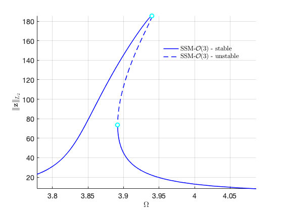
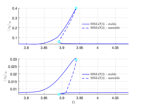
Verification using COCO
The following run uses the po-toolbox of COCO to calculate the forced reponser curve of the full system with collocation methods. It can take more than 10 minutes to finish.
coco = cocoWrapper(DS, nCycles, outdof2);
set(coco.Options, 'PtMX', 1000, 'NTST',20, 'dir_name', 'bd2');
set(coco.Options, 'NAdapt', 1, 'h_max', 200, 'MaxRes', 1);
coco.initialGuess = 'linear';
start = tic;
bd2 = coco.extract_FRC(freqrange);
timings.cocoFRCbd2 = toc(start)
 Run='bd2.FRC': Continue primary family of periodic orbits.

    STEP   DAMPING               NORMS              COMPUTATION TIMES
  IT SIT     GAMMA     ||d||     ||f||     ||U||   F(x)  DF(x)  SOLVE
   0                          1.19e-01  2.33e+02    0.0    0.0    0.0
   1   1  1.00e+00  5.85e-02  1.11e-05  2.33e+02    0.0    0.4    0.0
   2   1  1.00e+00  2.16e-04  4.57e-12  2.33e+02    0.1    0.7    0.1
   3   1  1.00e+00  4.79e-10  7.64e-14  2.33e+02    0.1    1.1    0.1

 STEP      TIME        ||U||  LABEL  TYPE         omega    po.period          eps         amp2         amp3
    0  00:00:06   2.3281e+02      1  EP      3.7796e+00   1.6624e+00   1.0000e+00   3.4609e-02   7.5810e-03
    6  00:00:45   2.7338e+02      2  EP      3.7782e+00   1.6630e+00   1.0000e+00   3.4638e-02   7.5780e-03

 STEP      TIME        ||U||  LABEL  TYPE         omega    po.period          eps         amp2         amp3
    0  00:00:46   2.3281e+02      3  EP      3.7796e+00   1.6624e+00   1.0000e+00   3.4609e-02   7.5810e-03
   10  00:01:58   3.6802e+02      4          3.7952e+00   1.6556e+00   1.0000e+00   3.4109e-02   7.6342e-03
   20  00:04:05   1.4265e+03      5          3.8635e+00   1.6263e+00   1.0000e+00   5.8904e-02   1.1201e-02
   30  00:07:01   2.3358e+03      6          3.9044e+00   1.6093e+00   1.0000e+00   1.8257e-01   2.0652e-02
   40  00:10:17   2.9264e+03      7          3.9307e+00   1.5985e+00   1.0000e+00   3.3978e-01   2.8199e-02
   47  00:13:25   2.9742e+03      8  SN      3.9357e+00   1.5965e+00   1.0000e+00   3.6912e-01   2.7578e-02
   50  00:14:06   2.9152e+03      9          3.9341e+00   1.5971e+00   1.0000e+00   3.5225e-01   2.4876e-02
   60  00:16:42   2.4434e+03     10          3.9164e+00   1.6043e+00   1.0000e+00   2.1776e-01   1.1419e-02
   70  00:19:07   1.5659e+03     11          3.8940e+00   1.6136e+00   1.0000e+00   8.0222e-02   6.3764e-03
   73  00:20:25   1.2081e+03     12  SN      3.8916e+00   1.6146e+00   1.0000e+00   5.6789e-02   6.4652e-03
   80  00:22:01   2.9151e+02     13          3.9467e+00   1.5920e+00   1.0000e+00   3.6105e-02   7.4960e-03
   82  00:22:29   1.1351e+02     14  EP      4.0866e+00   1.5375e+00   1.0000e+00   3.5941e-02   7.5450e-03

   Computation time:

   SSM based computation:    FRC_ep1:       34.1298
   Full system analysis:     cocoFRCbd1: 1.4807e+03
   SSM based computation:    FRC_ep1:       18.0423
   Full system analysis:     cocoFRCbd1: 1.3572e+03
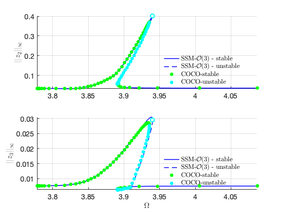
Primary resonance of the second mode
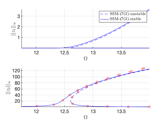
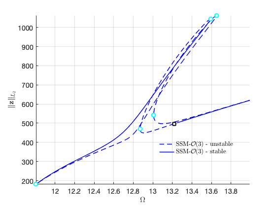
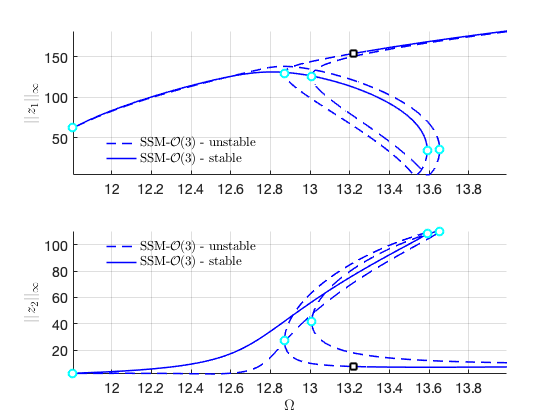
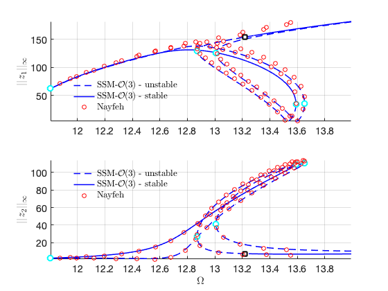
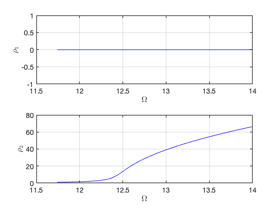
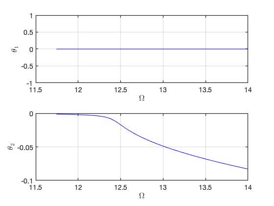
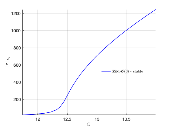
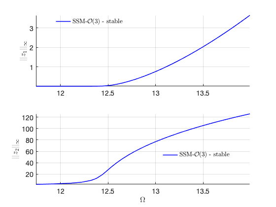
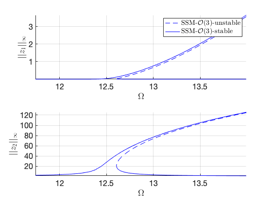
We move to the case that . Due to the internal resonance, there are two solution branches: one with trivial response for the first mode, and the other with nontrivial response for the first mode. In particular, the response of the system can be dominated by the contribution of the first mode due to the nontrivial branch.
We set and , .
c  = 10;
f = 40/epsilon;
n = 10;               % number of modes
Fext = zeros(n,1);    % excitation at modal coordinate
Fext(2) = f;
[mass,damp,stiff,fnl,fext] = build_model(c,Fext,epsilon,n);

% Create dynamical system
%

order = 2;
DS = DynamicalSystem(order);
set(DS,'M',mass,'C',damp,'K',stiff,'fnl',fnl);
set(DS.Options,'Emax',5,'Nmax',10,'notation','multiindex')
% Forcing
kappas = [-1; 1];
coeffs = [fext fext]/2;
DS.add_forcing(coeffs, kappas);
Getting nonlinearity coefficients
Loaded coefficients from storage
Linear Modal analysis
[V,D,W] = DS.linear_spectral_analysis();
Due to high-dimensionality, we compute only the first 5 eigenvalues with the smallest magnitude. These would also be used to compute the spectral quotients
Assuming a proportional damping hypthesis with symmetric matrices

modal damping ratio for 1 mode is 2.593810e-04
modal damping ratio for 2 mode is 8.004681e-05
modal damping ratio for 3 mode is 3.837148e-05
modal damping ratio for 4 mode is 2.243713e-05
modal damping ratio for 5 mode is 1.470421e-05

 The first 10 nonzero eigenvalues are given as
  -0.0010 + 3.8553i
  -0.0010 - 3.8553i
  -0.0010 +12.4927i
  -0.0010 -12.4927i
  -0.0010 +26.0610i
  -0.0010 -26.0610i
  -0.0010 +44.5690i
  -0.0010 -44.5690i
  -0.0010 +68.0077i
  -0.0010 -68.0077i
Choose Master subspace (perform resonance analysis)
S = SSM(DS);
set(S.Options, 'reltol', 1.0,'notation','multiindex');
resonant_modes = [1 2 3 4];
order = 3;
outdof = [1 2];
freqrange = [0.94 1.12]*imag(D(3));

set(S.FRCOptions, 'omegaSampStyle', 'cocoBD');
set(S.contOptions, 'h_max', 5, 'PtMX', 250);
set(S.FRCOptions, 'initialSolver', 'fsolve');
set(S.FRCOptions, 'coordinates', 'cartesian');
Non-zero (reproduce Nayfehs' solutions to get initial guess)
p0 = [imag(D(3));1];
z0 = [97.8562  -55.4066    1.9095    0.9820]'*1e3;
start = tic;
FRC_ep21 = S.SSM_isol2ep('isol2',resonant_modes, order, [1/3 1], 'freq', freqrange,outdof,{p0,z0});
timings.FRC_ep21 = toc(start)
The master subspace contains the following eigenvalues

lambda1 == - 0.001 + 3.8553i

lambda2 == (-0.001) - 3.8553i

lambda3 == - 0.001 + 12.4927i

lambda4 == (-0.001) - 12.4927i

sigma_out = 1
sigma_in = 1
Manifold computation time at order 2 = 00:00:00
Estimated memory usage at order  2 = 7.03E-02 MB
Manifold computation time at order 3 = 00:00:00
Estimated memory usage at order  3 = 1.03E-01 MB

Equation solved.

fsolve completed because the vector of function values is near zero
as measured by the value of the function tolerance, and
the problem appears regular as measured by the gradient.


 Run='isol2.ep': Continue equilibria along primary branch.

    STEP   DAMPING               NORMS              COMPUTATION TIMES
  IT SIT     GAMMA     ||d||     ||f||     ||U||   F(x)  DF(x)  SOLVE
   0                          3.33e-13  9.02e+01    0.0    0.0    0.0

 STEP      TIME        ||U||  LABEL  TYPE            om         Rez1         Rez2         Imz1         Imz2          eps
    0  00:00:00   9.0188e+01      1  EP      1.2493e+01   2.7697e+01   5.7009e+00  -5.5771e+01  -5.3928e-01   1.0000e+00
   10  00:00:00   7.1097e+01      2          1.2134e+01   1.7613e+01   2.1627e+00  -4.5439e+01  -3.1117e-01   1.0000e+00
   20  00:00:01   4.7482e+01      3  FP      1.1805e+01   3.6240e-02   1.0623e+00  -3.1405e+01  -1.2818e-01   1.0000e+00
   20  00:00:01   4.7482e+01      4  SN      1.1805e+01   3.6239e-02   1.0623e+00  -3.1405e+01  -1.2818e-01   1.0000e+00
   20  00:00:01   4.7482e+01      5          1.1805e+01   3.3801e-02   1.0623e+00  -3.1405e+01  -1.2818e-01   1.0000e+00
   30  00:00:01   5.2813e+01      6          1.1871e+01  -6.9363e+00   1.0265e+00  -3.4698e+01  -1.6226e-01   1.0000e+00
   40  00:00:01   9.5542e+01      7          1.2627e+01  -3.1241e+01  -6.1356e-01  -5.8545e+01  -5.6677e-01   1.0000e+00
   50  00:00:02   1.0318e+02      8          1.2789e+01  -3.4963e+01  -5.9400e+00  -6.2460e+01  -7.0314e-01   1.0000e+00
   60  00:00:02   1.0816e+02      9          1.3025e+01  -3.4834e+01  -2.4519e+01  -6.2149e+01  -1.4058e+00   1.0000e+00
   70  00:00:02   1.0509e+02     10          1.3340e+01  -2.9084e+01  -4.1800e+01  -5.2375e+01  -2.6528e+00   1.0000e+00
   80  00:00:03   9.2431e+01     11          1.3632e+01  -1.5476e+01  -5.5229e+01  -2.7928e+01  -3.9612e+00   1.0000e+00
   84  00:00:03   8.7811e+01     12  SN      1.3653e+01  -1.0121e+01  -5.6748e+01  -1.8138e+01  -4.0995e+00   1.0000e+00
   84  00:00:03   8.7811e+01     13  FP      1.3653e+01  -1.0121e+01  -5.6748e+01  -1.8138e+01  -4.0995e+00   1.0000e+00
   90  00:00:04   8.1284e+01     14          1.3583e+01   4.4564e-01  -5.5693e+01   1.2440e+00  -3.8940e+00   1.0000e+00
  100  00:00:04   8.2113e+01     15          1.3281e+01   1.6526e+01  -4.4549e+01   3.0491e+01  -2.6426e+00   1.0000e+00
  110  00:00:05   9.5052e+01     16          1.3023e+01   2.9096e+01  -2.5635e+01   5.3309e+01  -1.2971e+00   1.0000e+00
  113  00:00:05   9.9178e+01     17  FP      1.3008e+01   3.1396e+01  -2.0606e+01   5.7767e+01  -1.0874e+00   1.0000e+00
  113  00:00:05   9.9179e+01     18  SN      1.3008e+01   3.1396e+01  -2.0605e+01   5.7767e+01  -1.0874e+00   1.0000e+00
  120  00:00:05   1.1288e+02     19          1.3167e+01   3.5886e+01  -9.4725e+00   6.9414e+01  -8.9780e-01   1.0000e+00
  129  00:00:06   1.4165e+02     20  EP      1.3992e+01   3.8688e+01  -4.2808e+00   9.1210e+01  -1.2864e+00   1.0000e+00

 STEP      TIME        ||U||  LABEL  TYPE            om         Rez1         Rez2         Imz1         Imz2          eps
    0  00:00:06   9.0188e+01     21  EP      1.2493e+01   2.7697e+01   5.7009e+00  -5.5771e+01  -5.3928e-01   1.0000e+00
   10  00:00:06   9.7976e+01     22          1.2669e+01   3.1386e+01   1.0611e+01  -5.9502e+01  -7.2290e-01   1.0000e+00
   20  00:00:06   1.0462e+02     23          1.2942e+01   3.2764e+01   2.4662e+01  -6.0175e+01  -1.3654e+00   1.0000e+00
   30  00:00:06   1.0134e+02     24          1.3345e+01   2.6042e+01   4.4403e+01  -4.7942e+01  -2.8558e+00   1.0000e+00
   40  00:00:07   8.7514e+01     25          1.3589e+01   1.0846e+01   5.5677e+01  -2.0272e+01  -3.9602e+00   1.0000e+00
   41  00:00:07   8.6439e+01     26  FP      1.3590e+01   9.5210e+00   5.5908e+01  -1.7845e+01  -3.9772e+00   1.0000e+00
   41  00:00:07   8.6439e+01     27  SN      1.3590e+01   9.5210e+00   5.5908e+01  -1.7845e+01  -3.9772e+00   1.0000e+00
   50  00:00:08   7.8631e+01     28          1.3442e+01  -5.9668e+00   5.2474e+01   1.0442e+01  -3.4735e+00   1.0000e+00
   60  00:00:08   8.3883e+01     29          1.3096e+01  -2.1522e+01   3.7621e+01   3.8257e+01  -2.0208e+00   1.0000e+00
   70  00:00:08   9.7007e+01     30          1.2876e+01  -3.2181e+01   1.6800e+01   5.6747e+01  -9.0055e-01   1.0000e+00
   72  00:00:09   9.9243e+01     31  FP      1.2870e+01  -3.3367e+01   1.3361e+01   5.8872e+01  -8.1231e-01   1.0000e+00
   72  00:00:09   9.9244e+01     32  SN      1.2870e+01  -3.3368e+01   1.3358e+01   5.8873e+01  -8.1226e-01   1.0000e+00
   80  00:00:09   1.0945e+02     33          1.3012e+01  -3.6416e+01   4.3993e+00   6.6888e+01  -7.7030e-01   1.0000e+00
   85  00:00:10   1.1732e+02     34  HB      1.3216e+01  -3.7452e+01   3.1736e+00   7.2756e+01  -8.7405e-01   1.0000e+00
   90  00:00:10   1.4224e+02     35  EP      1.3992e+01  -3.9032e+01   2.4413e+00   9.1588e+01  -1.2833e+00   1.0000e+00

the forcing frequency 1.3992e+01 is nearly resonant with the eigenvalue -1.0000e-03 + i1.2493e+01
the forcing frequency 1.3916e+01 is nearly resonant with the eigenvalue -1.0000e-03 + i1.2493e+01
the forcing frequency 1.3782e+01 is nearly resonant with the eigenvalue -1.0000e-03 + i1.2493e+01
.
.
.
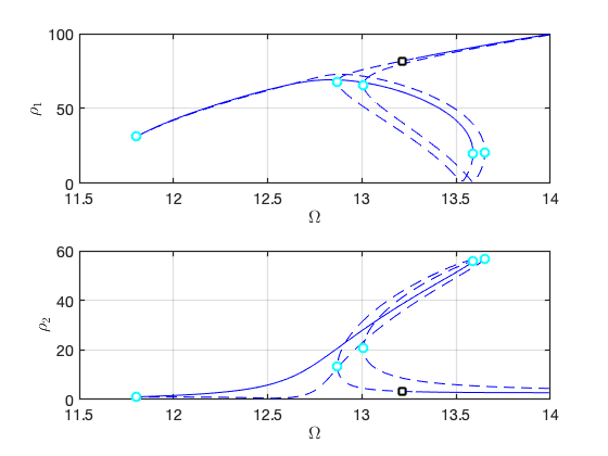
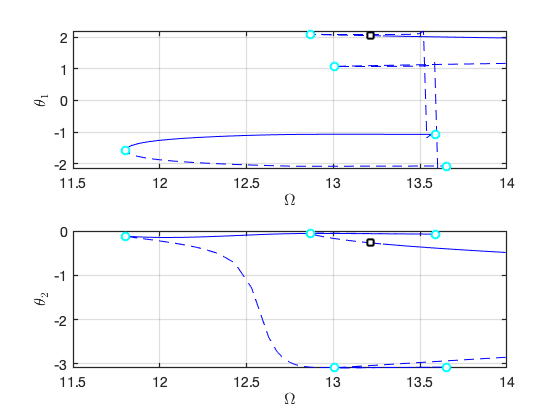
Load Nayfeh's solution for comparison
Nayfeh21 = load('NayfehSecondModeA1Nequal0.mat');
om2 = 12.4927;
omsamp = om2*(1+1e-4*Nayfeh21.SIG2);
figure(gcf); hold on
subplot(2,1,1)
plot(omsamp(1:150:end),Nayfeh21.A1(1:150:end),'ro','DisplayName','Nayfeh');
subplot(2,1,2)
plot(omsamp(1:150:end),Nayfeh21.A2(1:150:end),'ro','DisplayName','Nayfeh');
Zero upper branch
start = tic;
FRC_ep22 = S.SSM_isol2ep('isol3',resonant_modes, order, [1/3 1], 'freq', freqrange,outdof);
timings.FRC_ep22 = toc(start)
The master subspace contains the following eigenvalues

lambda1 == - 0.001 + 3.8553i

lambda2 == (-0.001) - 3.8553i

lambda3 == - 0.001 + 12.4927i

lambda4 == (-0.001) - 12.4927i

sigma_out = 1
sigma_in = 1

Manifold computation time at order 2 = 00:00:00
Estimated memory usage at order  2 = 7.03E-02 MB
Manifold computation time at order 3 = 00:00:00
Estimated memory usage at order  3 = 1.03E-01 MB

Equation solved.

fsolve completed because the vector of function values is near zero
as measured by the value of the function tolerance, and
the problem appears regular as measured by the gradient.


 Run='isol3.ep': Continue equilibria along primary branch.

    STEP   DAMPING               NORMS              COMPUTATION TIMES
  IT SIT     GAMMA     ||d||     ||f||     ||U||   F(x)  DF(x)  SOLVE
   0                          6.01e-13  2.58e+01    0.0    0.0    0.0

 STEP      TIME        ||U||  LABEL  TYPE            om         Rez1         Rez2         Imz1         Imz2          eps
    0  00:00:00   2.5757e+01      1  EP      1.2493e+01   0.0000e+00   1.3233e+01   0.0000e+00  -2.1882e-01   1.0000e+00
   10  00:00:00   1.7408e+01      2          1.2111e+01   0.0000e+00   2.0865e+00   0.0000e+00  -5.4386e-03   1.0000e+00
   13  00:00:00   1.6706e+01      3  EP      1.1743e+01   0.0000e+00   1.0674e+00   0.0000e+00  -1.4232e-03   1.0000e+00

 STEP      TIME        ||U||  LABEL  TYPE            om         Rez1         Rez2         Imz1         Imz2          eps
    0  00:00:00   2.5757e+01      4  EP      1.2493e+01   0.0000e+00   1.3233e+01   0.0000e+00  -2.1882e-01   1.0000e+00
   10  00:00:01   4.6394e+01      5          1.2781e+01   0.0000e+00   3.0183e+01   0.0000e+00  -1.1397e+00   1.0000e+00
   20  00:00:01   7.3740e+01      6          1.3354e+01   0.0000e+00   5.0298e+01   0.0000e+00  -3.1731e+00   1.0000e+00
   30  00:00:01   9.5637e+01      7  EP      1.3992e+01   0.0000e+00   6.5932e+01   0.0000e+00  -5.4679e+00   1.0000e+00

the forcing frequency 1.1743e+01 is nearly resonant with the eigenvalue -1.0000e-03 + i1.2493e+01
the forcing frequency 1.1771e+01 is nearly resonant with the eigenvalue -1.0000e-03 + i1.2493e+01
the forcing frequency 1.1924e+01 is nearly resonant with the eigenvalue -1.0000e-03 + i1.2493e+01
.
.
.
Zero lower branch
The fold point is outside the frequency span. So we calculate the lower branch directly with provided initial solution.
p0 = [1.06*imag(D(3));1];
z0 = [0 0 1 1]';
start = tic;
FRC_ep23 = S.SSM_isol2ep('isol4',resonant_modes, order, [1/3 1], 'freq',freqrange,outdof,{p0,z0});
timings.FRC_ep23 = toc(start)
The master subspace contains the following eigenvalues

lambda1 == - 0.001 + 3.8553i

lambda2 == (-0.001) - 3.8553i

lambda3 == - 0.001 + 12.4927i

lambda4 == (-0.001) - 12.4927i

sigma_out = 1
sigma_in = 1
Manifold computation time at order 2 = 00:00:00
Estimated memory usage at order  2 = 7.03E-02 MB
Manifold computation time at order 3 = 00:00:00
Estimated memory usage at order  3 = 1.03E-01 MB

Equation solved.

fsolve completed because the vector of function values is near zero
as measured by the value of the function tolerance, and
the problem appears regular as measured by the gradient.


 Run='isol4.ep': Continue equilibria along primary branch.

    STEP   DAMPING               NORMS              COMPUTATION TIMES
  IT SIT     GAMMA     ||d||     ||f||     ||U||   F(x)  DF(x)  SOLVE
   0                          1.55e-15  1.88e+01    0.0    0.0    0.0

 STEP      TIME        ||U||  LABEL  TYPE            om         Rez1         Rez2         Imz1         Imz2          eps
    0  00:00:00   1.8815e+01      1  EP      1.3242e+01   0.0000e+00  -1.0685e+00   0.0000e+00  -1.4262e-03   1.0000e+00
   10  00:00:00   1.8995e+01      2          1.2683e+01   0.0000e+00  -4.3654e+00   0.0000e+00  -2.3808e-02   1.0000e+00
   14  00:00:00   2.3222e+01      3  FP      1.2607e+01   0.0000e+00  -1.0497e+01   0.0000e+00  -1.3767e-01   1.0000e+00
   14  00:00:00   2.3229e+01      4  SN      1.2607e+01   0.0000e+00  -1.0504e+01   0.0000e+00  -1.3786e-01   1.0000e+00
   20  00:00:01   4.2333e+01      5          1.2775e+01   0.0000e+00  -2.7046e+01   0.0000e+00  -9.1490e-01   1.0000e+00
   30  00:00:01   6.9100e+01      6          1.3273e+01   0.0000e+00  -4.6937e+01   0.0000e+00  -2.7618e+00   1.0000e+00
   40  00:00:01   9.1344e+01      7          1.3879e+01   0.0000e+00  -6.2881e+01   0.0000e+00  -4.9705e+00   1.0000e+00
   42  00:00:01   9.4900e+01      8  EP      1.3992e+01   0.0000e+00  -6.5405e+01   0.0000e+00  -5.3803e+00   1.0000e+00

 STEP      TIME        ||U||  LABEL  TYPE            om         Rez1         Rez2         Imz1         Imz2          eps
    0  00:00:01   1.8815e+01      9  EP      1.3242e+01   0.0000e+00  -1.0685e+00   0.0000e+00  -1.4262e-03   1.0000e+00
    9  00:00:02   1.9827e+01     10  EP      1.3992e+01   0.0000e+00  -5.3399e-01   0.0000e+00  -3.5623e-04   1.0000e+00
the forcing frequency 1.3992e+01 is nearly resonant with the eigenvalue -1.0000e-03 + i1.2493e+01
the forcing frequency 1.3945e+01 is nearly resonant with the eigenvalue -1.0000e-03 + i1.2493e+01
the forcing frequency 1.3879e+01 is nearly resonant with the eigenvalue -1.0000e-03 + i1.2493e+01
.
.
.

Computation time:

SSM based computation:    FRC_ep1:       34.1298
Full system analysis:     cocoFRCbd1: 1.4807e+03
SSM based computation:    FRC_ep1:       18.0423
Full system analysis:     cocoFRCbd1: 1.3572e+03
SSM based computation:    FRC_ep21:      17.8259
SSM based computation:    FRC_ep22:       4.6606
SSM based computation:    FRC_ep23:       4.7044
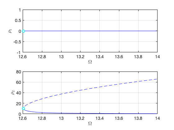
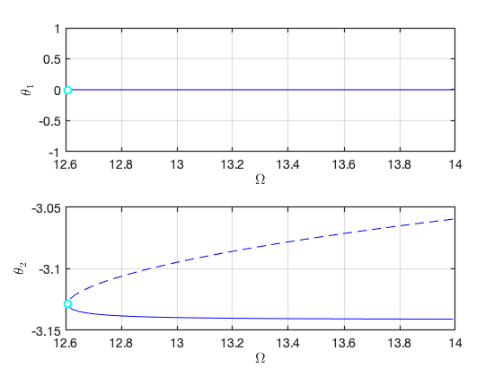
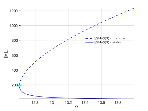
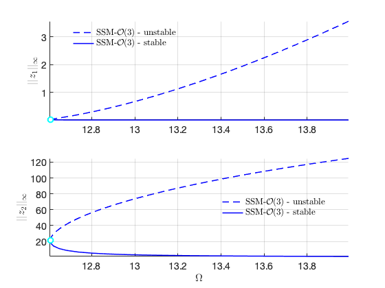
Plot the two branches in the same figure Here we have nonzero or in the equation of motion although due to the nonlinear mapping of SSM. In contrast, the method of multiple scale predcites that .
ST = cell(2,1);
ST{1} = {'b--','LineWidth',1.0}; % unstable
ST{2} = {'b-','LineWidth',1.0};  % stable
legs = 'SSM-$\mathcal{O}(3)$-unstable';
legu = 'SSM-$\mathcal{O}(3)$-stable';
figure;
subplot(2,1,1); hold on
plot_stab_lines(FRC_ep22.om,FRC_ep22.Aout_frc(:,1),FRC_ep22.st,ST);
plot_stab_lines(FRC_ep23.om,FRC_ep23.Aout_frc(:,1),FRC_ep23.st,ST,legs,legu);
xlabel('$\Omega$','Interpreter','latex');
ylabel('$||z_1||_{\infty}$','Interpreter','latex');
grid on; axis tight;set(gca,'FontSize',16)
subplot(2,1,2); hold on
plot_stab_lines(FRC_ep22.om,FRC_ep22.Aout_frc(:,2),FRC_ep22.st,ST);
plot_stab_lines(FRC_ep23.om,FRC_ep23.Aout_frc(:,2),FRC_ep23.st,ST);
xlabel('$\Omega$','Interpreter','latex');
ylabel('$||z_2||_{\infty}$','Interpreter','latex');
grid on; axis tight;set(gca,'FontSize',16)
Load Nayfeh's solution for comparison
Nayfeh21 = load('NayfehSecondModeA1equal0.mat');
om2 = 12.4927;
omsamp = om2*(1+Nayfeh21.epsilon*Nayfeh21.Sig2);
figure(gcf); hold on
subplot(2,1,2)
plot(omsamp(1:100:end),Nayfeh21.A2(1:100:end),'ro','DisplayName','Nayfeh');
