Stability Diagrams
Contents
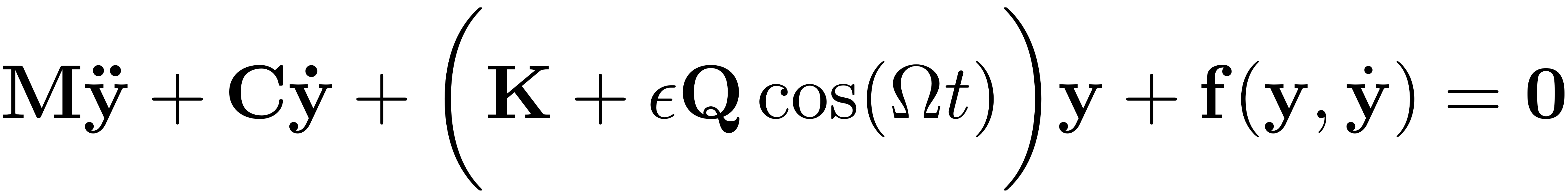
Consider a mechanical system of the type
Here,
 is a nonlinear function and
 is a linear matrix. This constitutes a generalised
 -dimensional Mathieu equation. The system is parametrically excited
with amplitude
-dimensional Mathieu equation. The system is parametrically excited
with amplitude
 . This excitation can destabilise the trivial fixed point with
 ,
,
 . The change of stability of this behaviour depending on the
excitation frequency
. The change of stability of this behaviour depending on the
excitation frequency
 and amplitude
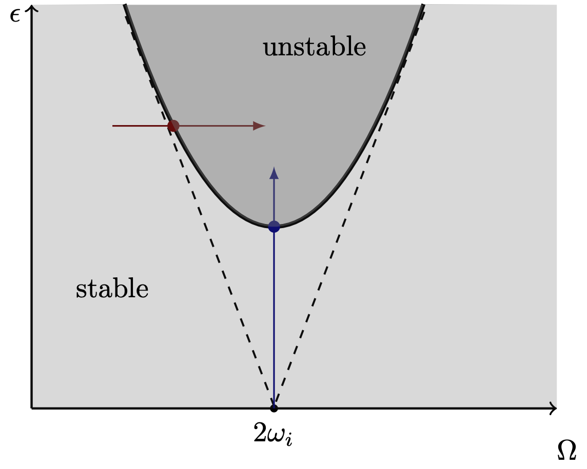
is commonly documented in a stability diagram. There, regions of
instability show up as resonance tongues, which occur when the
excitation frequency assumes subharmonic resonances with a mode of
the system. The resonance of main interest is the principal
parametric resonance where
and amplitude
is commonly documented in a stability diagram. There, regions of
instability show up as resonance tongues, which occur when the
excitation frequency assumes subharmonic resonances with a mode of
the system. The resonance of main interest is the principal
parametric resonance where

for some eigenfrequency
 of the mechanical system. By changing either the frequency or
amplitude, a bifurcation of the stability type is detected, when
crossing the boundary of the resonance tounge. Consequently families
of this bifurcation can be continued to get the resonance tongue
itself. As damping is decreased, it gets more pointed and closes in
to the
of the mechanical system. By changing either the frequency or
amplitude, a bifurcation of the stability type is detected, when
crossing the boundary of the resonance tounge. Consequently families
of this bifurcation can be continued to get the resonance tongue
itself. As damping is decreased, it gets more pointed and closes in
to the
 axis, as indicated by the dotted line.
To efficiently extract such resonance tongues, we compute the SSM
tangent to the
 -th modal subspace, to obtain an exact ROM for the dynamics of the
system. It serves as the ODE which is analysed using continuation
with
COCO.
Detailed treatment of the theory and algorithm can also be accessed
in the related publication (Thurnher, Haller & Jain, 2023).
-th modal subspace, to obtain an exact ROM for the dynamics of the
system. It serves as the ODE which is analysed using continuation
with
COCO.
Detailed treatment of the theory and algorithm can also be accessed
in the related publication (Thurnher, Haller & Jain, 2023).
After setting up the dynamical system, and the SSM object
S, the boundary region of stable response can be
detected by using the following built-in method:
SD = S.extract_Stability_Diagram(resModes, order, OmegaRange,epRange,'amp', p0,'PD',PlotSD);
The input arguments are as follows
-
resModesis an array which indicates the 2D master subspace, which is in 2:1 resonance with the parametric excitation. -
orderdenotes the order of the non-autonomous SSM approximation which is to be computed. -
OmegaRangedenotes the frequency range over which the diagram should be extracted. -
epRangedenotes the excitation amplitude range for which the diagram should be constructed. Note that SSM-theory is local in nature, and that it computes asymptotic series expansions in this parameter - so this parameter may not be chosen to be arbitrarily large. -
'amp'or'freq': which indicates the initial parameter which should be chosen for continuation - see the figure above for reference. -
p0: an initial set of parameters for finding the location of the resonance tongue. For small excitation frequencies and low damping parameters, the initial guess for
should be chosen to be zero for fast convergence.
-
'PD'or'SN': depending on which parameter is chosen, the tongue is sought in terms of period-doubling or saddle-node bifurcations. See the explanation below -
PlotSD: a boolean parameter for plotting the result of the computation.
Saddle-Node and Period-Doubling Bifurcations
We write the mechanical system in the standard form. By extending the resulting dynamical system

to an autonomous system of variables
 the trivial fixed point
 of the paremtrically excited system can be interpreted as the
periodic orbit
of the paremtrically excited system can be interpreted as the
periodic orbit
 . Any change of the stability behaviour of this periodic orbit is
then given by some bifurcation. At the stability boundary of the
principal resonance with
. Any change of the stability behaviour of this periodic orbit is
then given by some bifurcation. At the stability boundary of the
principal resonance with
 nontrivial periodic orbits with response period
 emerge. If continuation of
 periodic orbits is used then these bifurcations show up as period
doubling ('PD') bifurcations. Initially continuing
periodic orbits is used then these bifurcations show up as period
doubling ('PD') bifurcations. Initially continuing
 periodic orbits leads to a saddle node ('SN') bifurcation. The
function extract_Stability_Diagram allows to chose between these two
options for constructing the stability diagram.
periodic orbits leads to a saddle node ('SN') bifurcation. The
function extract_Stability_Diagram allows to chose between these two
options for constructing the stability diagram.
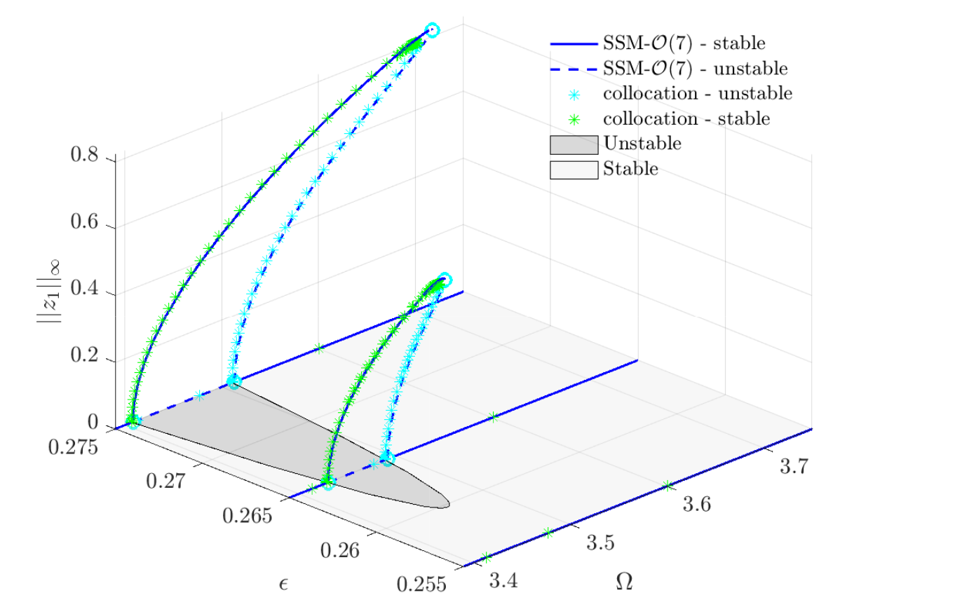
Emergent response
The boundary region of unstable response is at the same time a branch point, from which non-trivial periodic orbits emerge. An illustration of this is shown in the following figure, which shows the response for a 2-dimensional, nonlinear Mathieu equation. The response obtained from the ROM provided by the dynamics on the SSM is verified using collocation on the full dynamical system: